
CHAPTER
COORDINATORS
COORDINATORS
Fujiang Yu
7.2
Storm surge modelling

7.2.1
Architecture components and singularities
Storm surge models are generally based on the two-dimensional shallow water equation to compute the water level and velocity. According to different modelling purposes, the storm surge model can be divided into: i) storm surge model without tide; ii) storm surge model including astronomical tide; and iii) storm surge flooding model considering inundation.
In a storm surge model without tide, only the effect of the meteorological forcing needs to be considered. Obtained result is only the water level rising and falling under the effect of atmospheric pressure and wind. The role of this model is generally to provide forecasters with a reference for the magnitude of storm surge when making forecasts, and it cannot truly reflect the fluctuations of water level.
Based on the former model, the tidal boundary conditions and tidal potential are introduced in the total water level storm surge model, in which the nonlinear interaction between storm surge and astronomical tide can be fully considered in the model. This model can be used for releasing storm surge numerical forecast products and providing reference for coastal response to storm surge disasters. It can also provide the water level changes in the target area under the influence of extreme weather conditions for coastal engineering (such as harbours, wharfs, seawalls, offshore wind farms, etc.).
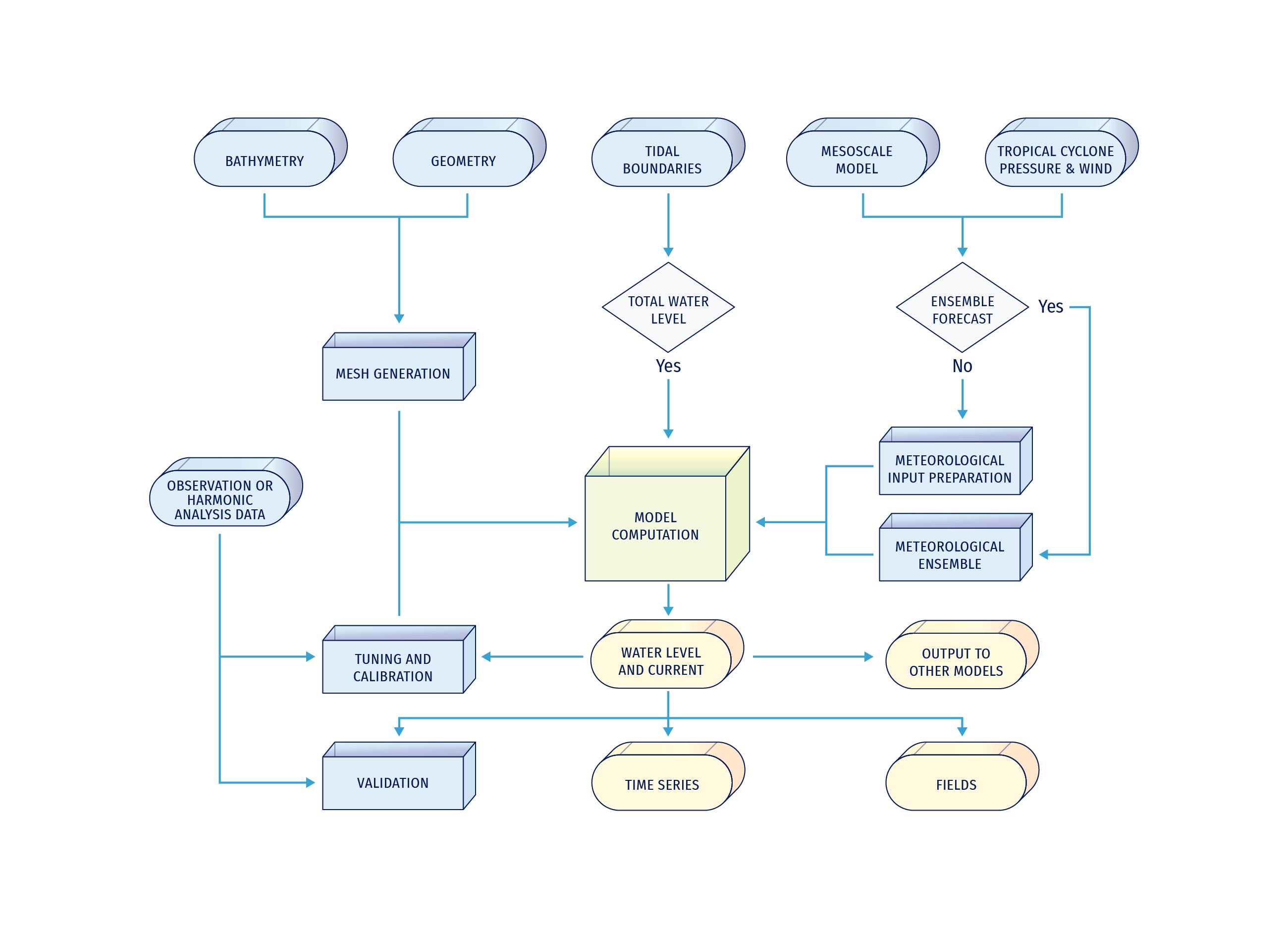
Figure 7.9. Storm surge modelling flow chart.
The storm surge flooding model considering inundation is more complicated than the previous two models. The interaction of storm surge and astronomical tide, and the interaction of storm surge and wave are also considered in the model. The inundation range and depth of the coastal area can be obtained by a storm surge simulation. Figure 7.9 shows the main storm surge modelling components used by a forecasting system and that will be detailed in the next sections.
7.2.2
Input data: available sources and data handling
7.2.2.1
Bathymetry and geometry
Reliable and accurate shoreline and bathymetry data are the basis for modelling of storm surge, tidal, and storm surge flooding models. In the process of model setup, the computational grid should be determined according to the demand, and then the data of shoreline and bathymetry should be collected according to the location and scope.
Sources of bathymetric data can be found on Section 4.2.4. These data need to be used with caution when establishing high-resolution storm surge models. As the bathymetry of coastal or estuary changes rapidly over time, these upstream data may not be able to be updated in time. Therefore, the correctness of the data needs to be verified before it is used.
When the published upstream data do not meet the requirements, it is preferable to use the latest sea chart or high-resolution DEM data. In addition, the datum of the data needs to be confirmed as, due to different sources of data, the datum could be different. In order to truly reflect the effects of bathymetry on storm surges, data from different sources need to be unified on the same datum.
7.2.2.2
Tidal boundaries
In the storm surge and storm surge flooding modelling, tidal waves are generally used as open boundary conditions. Open boundary conditions can be velocity, water level, or harmonic constant.
Tidal height at any location and time can be written as a function of harmonic constituents according to the following general relationship:

Where:
- H(t) = height of the tide at any time t
- Ho= mean water level above some defined datum such as mean sea level
- Hn = mean amplitude of tidal constituent n
- fn= factor for adjusting mean amplitude Hn values for specific times
- an = speed of constituent n in degrees/unit time
- t = time measured from some initial epoch or time, i.e., t=0 at to
- (Vo+ u)n = value of the equilibrium argument for constituent n at Greenwich and when t=0
- gn= epoch of constituent n, i.e., phase shift from tide-producing force to high tide from to
In Eq. 7.1, for a tidal component, the fn and the (Vo+ u)n will change with time, and the Hnand the gnwill change with the geographical location. Therefore, according to the start time of simulation, the fn and (V0+ u)n of the proposed tidal component should be set in the model, and the Hn and the gn boundary conditions should be given according to the position of the boundary grid node.
The location of the tidal open boundary is critical. First of all, it is necessary to ensure that the grid can completely cover the definition area. Secondly, it is better to set the open boundary near the tidal station, because the tidal constituent data near the tidal station is more accurate. Finally, it is preferable not to set the open boundary at the amphidromic point nearby, because too small amplitude will bring uncertainty to the simulation.
The data for tidal boundaries can be obtained by downloading publicly available data on tidal harmonic constants covering most of the oceans. TPXO (Egbert et al., 1994; Egbert and Erofeeva, 2002) is a widely used global tidal data. It is a series of fully global models of ocean tides, which best fits, in a least squares sense, the Laplace Tidal Equations and altimetry data. The TPXO models include eight primary (M2, S2, N2, K2, K1, O1, P1, Q1), two long period (Mf, Mm) and 3 non-linear (M4, MS4, MN4) harmonic constituents (plus 2N2 and S1 for TPXO9 only). More detailed information can be found at 🔗2). In addition, also the NAO.99b tide model (Matsumoto et al., 2000 and 2001), which is developed by assimilating TOPEX/POSEIDON Altimeter Data into Hydrodynamical Model, can provide global tide data. This model provides 16 short-period harmonic constituents (M2, S2, K1, O1, N1, N2, P1, K2, Q1, M1, J1, OO1, 2N2, Mu2, Nu2, L2, L2, and T2), 7 long-period harmonic constituents (Mf, Mm, Msf, Msm, Mtm, Sa, Ssa) data with of 0.5 degrees, and provides 16 short-period harmonic constants around Japan with a resolution of 5 minutes. More detailed information can be found at 🔗3.
Once the model and tidal boundaries have been established, they need to be tuned and calibrated before using. The model can be run with tidal boundaries and tidal potential. The tidal results are more sensitive to changes in the bottom friction coefficient and the bathymetry. By calibrating the tidal simulation, a reasonable bottom friction coefficient can be set for the model. At the same time, the difference in the tidal results caused by the bathymetry from dissimilar sources helps to find more suitable bathymetry data for the model.
7.2.2.3
Meteorological inputs
In storm surge or storm surge flooding modelling, the input from meteorological forcing mainly includes surface wind shear stress and atmospheric pressure at sea surface level. In deep water, the sea level rises are mainly caused by the atmospheric pressure gradient, i.e. the water level rises approximately 1 cm at every reduction in pressure of 1 mbar. In shallow water, estuary and nearshore, wind shear stress is the dominant force of the storm surge, and the sea level rise is proportional to the square of wind speed. Therefore, accurate meteorological inputs, especially sea surface wind, is essential for storm surge modelling. The accuracy of storm surge results depends largely on the quality of meteorological data.
Depending on the storm surge modelling purposes, the types of meteorological forcing input are different. At present, there are two main sources of wind field for storm surge modelling: atmospheric model and empirical formula. Atmospheric models can provide global or regional meteorological fields; the main elements required for storm surge calculation are sea level pressure and 10 metres wind. The horizontal resolution of these data is between ten and tens of kilometres, and the forecast period can reach up to 240 hours. This kind of meteorological field is mainly used in the calculation of storm surge caused by extratropical cyclones. Compared with extratropical cyclones, tropical cyclones are smaller in scale but stronger in intensity, and atmospheric models cannot resolve the structure of tropical cyclones well. Therefore, the meteorological field from atmospheric models is not applicable to the typhoon storm surge calculation. Empirical formulas for tropical cyclone pressure and wind are often applied to create meteorological forcing fields for tropical storm surge models. Since the wind speed and pressure structure of tropical cyclones are close to axisymmetric, their distribution can be reasonably represented with an empirical formula for the radial distribution of wind or pressure.
The commonly used empirical formulas for pressure distribution mainly include the following:
Takahashi (1939):
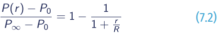
Myers (1954):
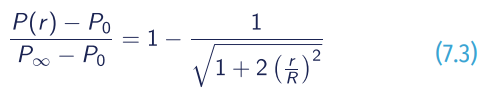
Myers (1954):

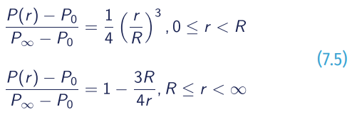
Jelesnianski (1965):
Bjerknes (1921):
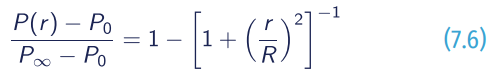
Holland (1980):
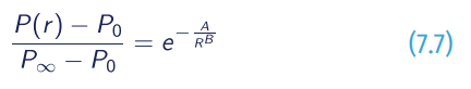
Where:
- P∞= the ambient pressure;
- Po = the pressure at the tropical cyclone centre;
- P(r) = the pressure at r from tropical cyclone centre;
- A and B = empirical parameters that control the tropical cyclone size.
The tropical cyclone wind field is formed by the superposition of two vector fields (Ueno, 1981). The first vector field is a wind field symmetrical to the centre of the cyclone. The wind vector passes through the isobar and points to the left with a 20° deflection angle.
The wind speed is proportional to the gradient wind, which can be expressed by the following formula:
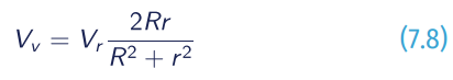
- Vr = the maximum wind speed;
- R = the radius of the maximum wind.
The second vector field caused by the movement of cyclone is superimposed on the wind system for the stationary symmetric cyclone, and that the wind velocity V→f is:
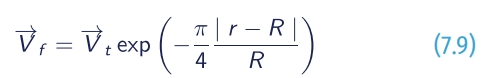
- V→t = velocity of typhoon;
- R = the radius of the maximum wind.
Consequently, the wind velocity W→ is:

The typhoon centre pressure, maximum wind speed, moving speed and other parameters can be obtained from websites of national meteorological agencies.
7.2.3
Modelling component
7.2.3.1
Governing equations
The governing equations of numerical simulation were determined by the flow dynamic theory.
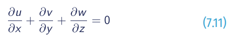
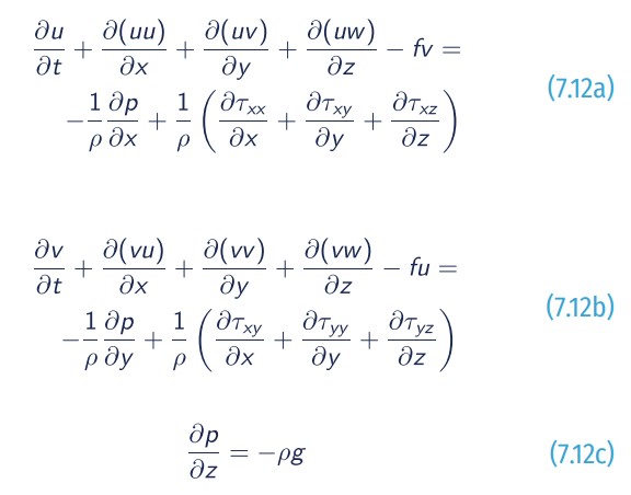
The three-dimensional flow equations are as follows:
- Continuity equation:
- Momentum equation:
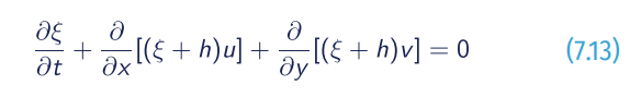
Based on hydrostatic approximations and incompressible assumption of fluid, the depth integrated two-dimensional storm surge governing equations can be written as:
- Continuity equation:
- Momentum equation:
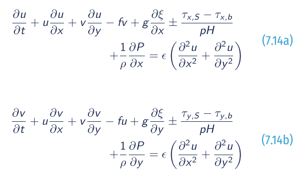
Where:
- ξ= free surface elevation relative to the geoid;
- h = water depth;
- f = Coriolis coefficient;
- ρ = density of water;
- g = gravitational acceleration;
- (τx,S , τx,b) = free-surface shear stress in x and y direction;
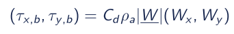
- W_ = wind speed at 10 metres above sea surface;
- Wx , Wy = wind speed components in x and y direction;
- Cd = wind Drag coefficient which is relevant to wind speed;
- τx,b, τy,b = bottom shear stress in x and y direction;
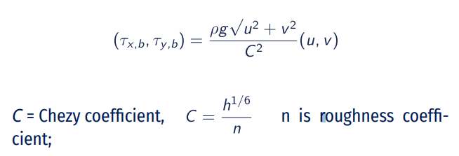
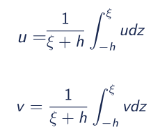
- u, v = depth-averaged horizontal velocity components in x and y direction;
- P = atmospheric pressure at the free surface;
- ε = depth-averaged horizontal eddy viscosity.
7.2.3.2
2D barotropic and 3D baroclinic models for storm surge
Hydrodynamic models are generally divided into vertically averaged 2D barotropic, 3D barotropic, or 3D baroclinic models. These types of models can be used for storm surge modelling. Minato (1998) first studied the effect of a 3D model on storm surge results and simulated the water level change caused by Typhoon 7010 in Tosa Bay, Japan. The results showed that the difference between the 3D model and the 2D model is about 2 to 10%. Weisberg and Zheng (2008) found that under the condition of setting the same bottom friction coefficient, the 3D model simulates higher extreme water level than the 2D model. Subsequently, simulating the storm surge of Hurricane Ike in the Gulf of Mexico, Zheng et al. (2013) pointed out that the 2D and the 3D models have differences in the trend and peak values of water level, but the calibration of the bottom friction is more important. Ye et al. (2020) studied the influence of baroclinic models on storm surge simulation results. Sensitivity tests show that the impact of the baroclinic model on storm surge is not significant, but it has a greater impact on current.
Since the vertical velocity distribution structure of the 2D model is different from that of the 3D model, the vertical average velocity is greater than that near the bottom layer, so that the bottom shear stress of the 2D model will be greater. Satisfactory results can be obtained for both types of models by calibrating the bottom friction.
Regarding operational storm surge modelling, computational efficiency is a factor that must be considered. 3D models generally divide the water body into multiple layers vertically, so they require more computing time than 2D models. If the purpose of storm surge modelling is to obtain water level, rather than currents, the 2D models are the best choice for balancing calculation efficiency and accuracy. Most of the existing operational storm surge forecasting systems are 2D models.
7.2.3.3
Wetting and drying scheme
During the simulation of storm surge inundation, the grid points close to the coastline in the model will be either wet or dry due to the fluctuation of water level. Therefore, the model needs to determine the dry and wet state of a grid point according to the state of the surrounding grid points.
Assuming that the state of a certain grid point is wet, if the calculated water level makes the water volume less than zero, then this grid point will become a dry grid point and will not participate in the next calculation. In practical calculations, to prevent the negative value of the water volume at a grid point, which makes the momentum equation and continuity equation meaningless, a threshold value greater than zero is usually selected. When the water volume is less than the threshold value, the state of the grid point is defined as dry.
Assuming that the state of a certain grid point is dry, the first step is to check how many of the surrounding grid points are wet grid points. If more than one is wet grid point, then the water level is averaged over these wet grid points. If the averaged water level is greater than the threshold water level, the state of this grid point may become wet, otherwise it still remains as a dry one. In the second step, it is necessary to further check the transport over the cross-section area between the grid point and the surrounding wet grid points. If these transport cross-section areas are all positive, then the dry grid point becomes a wet grid point and participates in the next calculation; otherwise, it is still a dry grid point.
7.2.3.4
Grid types
The grids used in most sea level models are mainly divided into two categories: structured and unstructured grids. The structured grid nodes are arranged in an orderly manner, and the connection relationship between adjacent nodes is fixed. In contrast, the unstructured grid nodes are arranged in an unordered manner and the adjacent nodes have no fixed connection relationship. Differently from structured grids, unstructured grids with triangular elements allow to adjust the resolution flexibly to depict complex shapes of coastline and estuary (Figure 7.10).
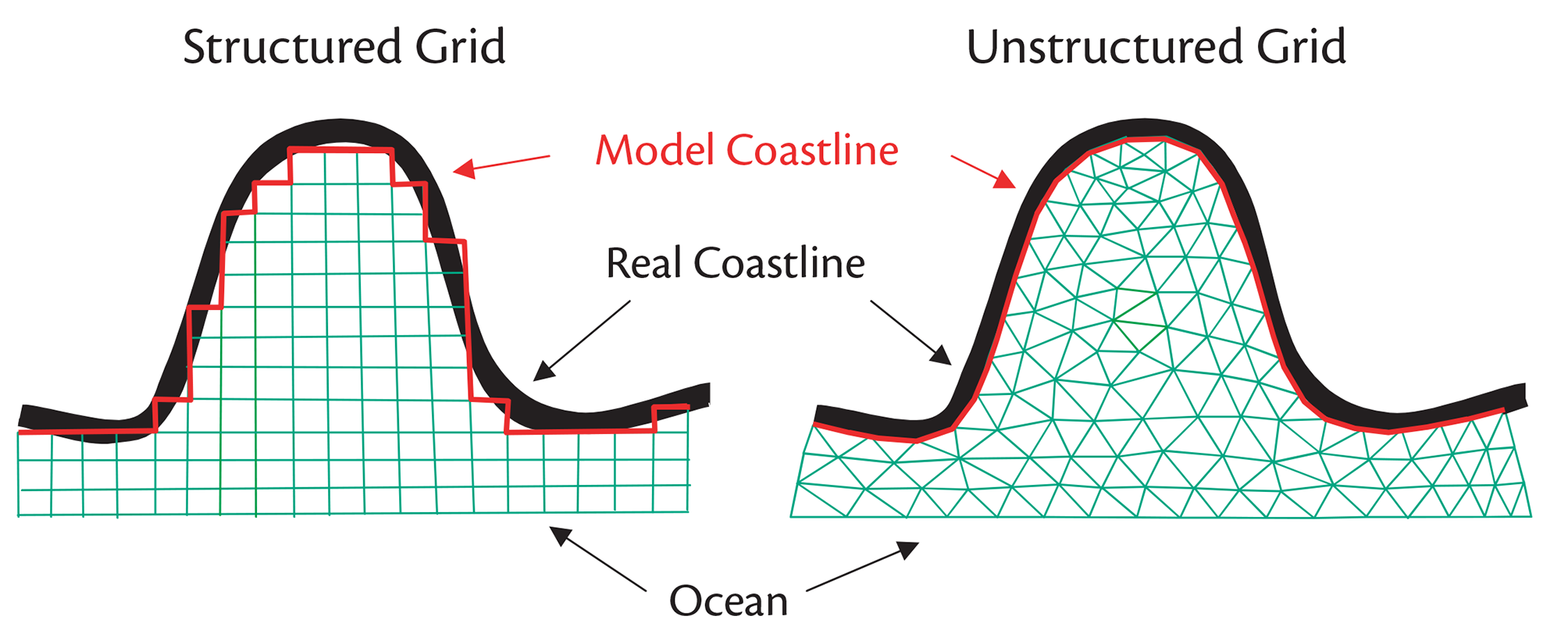
Figure 7.10. Structured grid and unstructured grid at coastal area.
Structured grids mainly have two forms: rectangular grids and curvilinear grids. Relatively speaking, the curvilinear grid can adapt better to the complex shape of the coastline, and it can also realise the change of grid resolution that is more advantageous for storm surge simulation in estuary area (Figure 7.11).
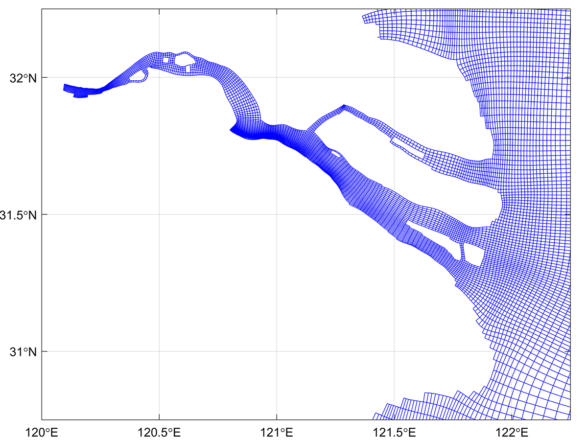
Figure 7.11. An example of curvilinear grid.
Triangular grids were the main forms of unstructured grids until a new form of unstructured grids, the SCVTs (Figure 7.12), appeared in ocean modelling a decade ago (Ringler et al., 2013). Like the triangular grids, the SCVTs can adapt well to complex coastline, and facilitate a smooth transition from coarse resolution grid cell to high resolution grid cell. In addition, they also solve the computational instability problem caused by small acute angles in the triangular grid. At present, the SCVTs model has been used in the China Sea (as shown in Figure 7.13)
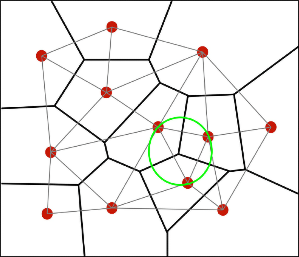
Figure 7.12. An example of Voronoi tessellation schematic diagram: centroid in red, Voronoi circle in green, edges in grey.
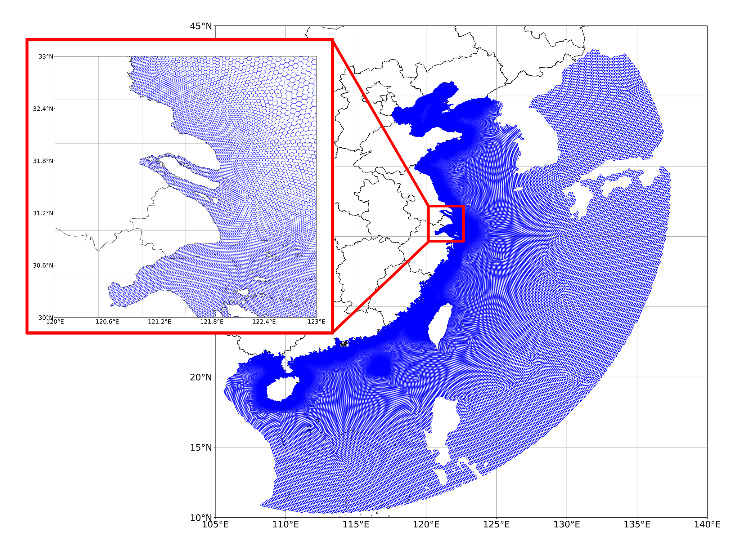
Figure 7.13. A storm surge model grid based on SCVTs applied to the China Sea.
7.2.3.5
Discretization method
The main discretization methods include finite difference method, finite element method, and finite volume method. Discretization methods also correspond to the types of grids used. The finite difference method is generally used for structured grids, while the finite element method and finite volume method are generally used for unstructured grids.
The FDM is one of the simplest and oldest methods to solve the storm surge problems, and it is still widely used. This method divides the solution domain into differential grids, replacing the continuous solution domain with a finite number of grid nodes. By using the Taylor series expansion, the derivative of the governing equation is discretized by the difference quotient of the function value on the grid node, so as to establish the algebraic equations with the value on the grid node as the unknown quantity. This method is an approximate numerical solution that directly transforms a differential problem into an algebraic problem. The mathematical concept is intuitive and simple to express. It is an earlier and relatively mature numerical method.
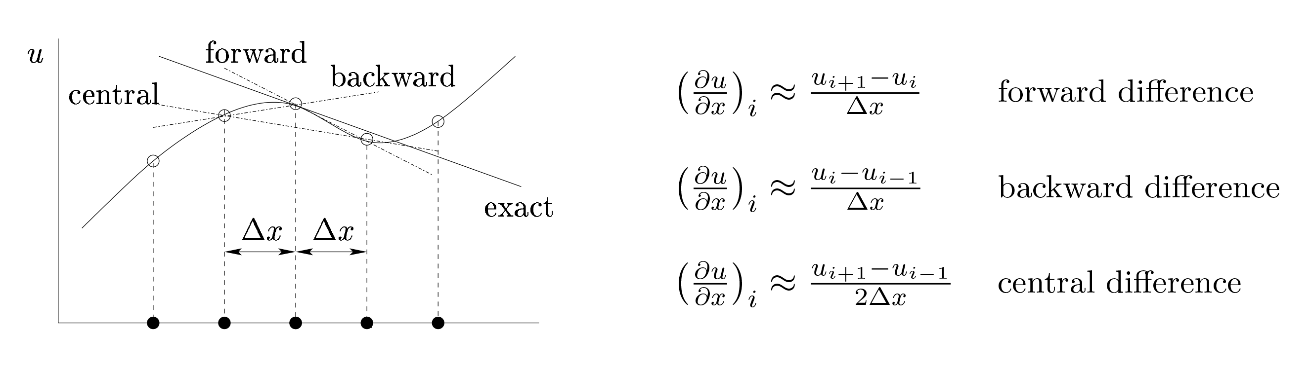
Figure 7.14. Geometric interpretation of difference expression.
The basic difference expression mainly has three forms (Figure 7.14): forward difference, backward difference, and centre difference. The first two formats are first-order derivatives, while the last format is second-order derivatives. Different computational schemes can be obtained through the combination of several different formats of time and space.
According to the precision of the scheme, we can distinguish among first-order, second-order, and high-order accuracy schemes. Depending on the influence of the time factor, the difference scheme can also be divided into explicit scheme, implicit scheme, explicit and implicit alternate scheme.
The FEM is based on variational principle and weighted residual method. The basic solution idea is to divide the computational domain into a finite number of non-overlapping elements. In each element, some appropriate nodes are selected as interpolation points of the solution function. The variable in the differential equation is changed into a linear expression composed of the node value of each variable or its derivative and the selected interpolation function. The differential equation is solved discretely by means of variational principle or weighted residual method.
According to the difference of the weight function and the interpolation function, the finite element method is divided into several computational schemes. For the choice of weight function, there are collocation methods, moment method, least square method, and Galerkin method. According to the shape of the computing cell grid, there are triangular grid, quadrilateral grid, and polygonal grid. Triangular grids are commonly used in storm surge modelling. The accuracy of the interpolation function is divided into linear interpolation functions and high-order interpolation functions. Different combinations also constitute different finite element calculation schemes.
The FVM is also called the control volume method. The basic idea is to divide the computational domain into a series of non-overlapping control volumes, and make a control volume around each grid point. Integrate the differential equations to be solved for each control volume to obtain a set of discrete equations. The unknown is the value of the dependent variable at the grid point. In order to obtain the integral of the control volume, it is necessary to assume the changing law of the value between grid points, i.e. the distribution profile (continuous or segmented) of the assumed value. From the selection method of the integral region, the finite volume method belongs to the subregion method in the weighted residual method. From the approximate method of the unknown solution, the finite volume method is a discrete method using local approximation. The physical meaning of the discrete equation is the conservation principle of the dependent variable in a finite controlled volume, just as the differential equation expresses the conservation principle of the dependent variable in an infinitely small controlled volume. The discrete equation obtained by the finite volume method requires the integral conservation of the dependent variable to be satisfied for any set of control volumes, and naturally also for the entire computation area. This is the attractive advantage of the finite volume method. Some discrete methods, such as the finite difference method, only satisfy the integral conservation if the grid is extremely fine. The finite volume method shows accurate integral conservation even in the case of coarse grids. As far as the discrete method is concerned, the finite volume method can be regarded as an intermediate between the finite element method and the finite difference method.
7.2.3.6
Existing models for storm surge modelling
Numerical simulation of storm surges began in the 1950s. After decades of development, it has emerged that many numerical models can be used to storm surge simulations. Commercial models include MIKE21 and TuFlow, while examples of free models are: ADCIRC, Delft3D-FLOW, POM, FVCOM, ROMS, and SCHISM. Free numerical models generally provide the source code of the model, so that the model can be modified as needed when establishing a forecasting system. The models listed in Table 7.1.can be used to establish a complete operational storm surge forecasting system.
| Model | Grid topology | Numerical methods | Nesting capabilities | Website |
|---|---|---|---|---|
| MIKE21 | Structured curvilinear grid and unstructured grid | Alternating direction implicit method for structured grid. Cell-centered finite volume method for unstructured grid | Nesting is not possible | https://www.mikepoweredbydhi.com/products/mike-21-3 |
| TuFlow | Structured grid and unstructured grid | 2nd order semi-implicit matrix solver for structured grid. Finite-Volume for unstructured grid | Sub-Grid | https://www.tuflow.com/ |
| ADCIRC | Unstructured grid | Finite element method in space and finite difference method in time | Not available | https://adcirc.org/ |
| Delft3D-FLOW | Structured curvilinear grid | Alternating direction implicit method | Nested boundary conditions | https://oss.deltares.nl/web/delft3d/ |
| POM | Structured curvilinear grid | Finite difference scheme | Not available | http://www.ccpo.odu.edu/POMWEB/index.html |
| FVCOM | Unstructured grid | Finite volume method | Nesting at the boundaries | http://codfish.smast.umassd.edu/fvcom/ |
| ROMS | Structured curvilinear grid | Second-order finite differences | One-way nesting | https://www.myroms.org/ |
| SCHISM | Unstructured mixed triangular/ quadrangular grid | Semi-implicit Galerkin finite element method | One-way nesting | http://ccrm.vims.edu/schismweb/ |
Table 7.1. Geometric interpretation of difference expression.
7.2.4
Data assimilation systems
Data assimilation techniques are used to combine model and observed data to obtain the best estimate of the state of a system (see Chapter 4.3 for more details). Statistical techniques are often employed to find a solution which, ideally, minimises some error metric. For storm surges, this is done to obtain fields of sea surface height that can help us to better understand past events or to improve the quality of forecasts. An overview of the application of data assimilation to storm surge modelling and forecasting is provided in this section. Henceforth, references to errors mean some metric distance between the model and observations.
7.2.4.1
Sources of error in storm surge models
In order to reduce errors in storm surge models, especially for forecasting in which the accuracy may influence real-time decision making, it is important to understand the sources of error. Some of the main sources are given below.
Quality of input datasets
This includes atmospheric surface forcing and tidal forcing at the boundaries (see Section 7.2.2). Storm surges are largely forced phenomena; therefore, the accuracy of forcing is key and errors in the related datasets may be transferred into the storm surge component of the modelled sea surface height. Errors in input datasets may arise from similar sources as the storm surge model, including model and instrument errors.
For example, errors in tidal amplitudes and phases at the boundaries will propagate with the tidal waves into the domain. As discussed in Section 7.2.1, interactions with the tides can influence both timing and height of a storm surge, so it is important to have an accurate tidal component in the model. The accuracy of the surface atmospheric forcing is important as well, especially the components of wind and surface pressure. Due to the forced nature of storm surges, this is one of the largest sources of error in storm surge forecasts (Horsburgh et al., 2011).
Tuning of model parameters
It is common practice to adjust various model parameters to obtain a better solution. For example, it could include the tuning of bottom/surface friction coefficients. It is very unlikely to find a perfect parameter set, and the iterative processes often used can lead to non-optimal solutions. See Section 7.2 for more information about parameters used in storm surge models.
Representativity errors
Representativity errors arise from models’ ability to represent variables and processes such as resolution (Daley, 1991). For example, a coarse model may not be able to resolve finer scale features, which is present in the observations. For storm surges, this is particularly important nearby complex coastlines and estuaries. Similarly, coarser models may mean smoother bathymetry in these areas, which can significantly affect the modelled surge.
A model may not simulate all processes required to accurately model a storm surge. For example, if tides are not included in the model, only the atmospherically forced component of sea surface height is being generated, and contributions from tide-surge interactions will be missing. Other examples include the lack of tidal processes such as self-attraction and loading, or not including the inverse barometer effect in the model.
7.2.4.2
Assimilated data sources for storm surge modelling
An attempt to reduce the impact of the errors described in the previous section can be made using data assimilation. For storm surge modelling, assimilation of observations may occur directly into the model or indirectly via input datasets.
Datasets used as atmospheric forcing often contain assimilated observations. The generation of the storm surge is highly dependent on the model’s interaction with these datasets and it is vital that they are accurate. For example, the forecasted atmospheric fields used at the UK Met Office use assimilation of atmospheric observations. There are also many reanalysis datasets available, such as the ECMWF ERA5 dataset (Hersbach et al., 2020) that assimilates observations from multiple sources to generate atmospheric data. While these examples are suitable for extratropical storm surges, they may not sufficiently resolve intense tropical cyclones, meaning that parametric methods may be a better option (see Section 7.2.2.3). There are also assimilative alternatives, such as the MTCSWA datasets (Knaff et al., 2011), which blend together parametric fields and observations. These have been shown to have some benefit for forecasting (Byrne et al., 2017). The same is true for the datasets used to derive tidal signals at the model boundaries. Examples of such datasets include TPXO (Egbert et al., 2002) and FES (Lyard et al., 2021), which incorporate data from satellite altimetry and tide gauges. See Section 7.2.2.2 for more information on these tidal datasets.
Sea surface height may also be assimilated directly into the modelled sea surface. There are two sources used, both with advantages and disadvantages: tide gauges and satellite altimetry. Tide gauges (and other fixed instruments such as bottom pressure recorders) offer information that is frequent and consistent in time, making them useful for capturing ocean processes of all frequencies (including storm surges). However, they are generally spatially sparse. On the other hand, altimetry data offer good spatial coverage but are less consistent in time, as a satellite only returning to the same location once every number of days. This makes the data useful for longer periods of periodic ocean processes.
Tide gauge data are currently assimilated for storm surge forecasting at some institutions (see Section 7.2.4.4). There are representativity challenges that must be considered when using these data. Most importantly, modelled sea surface height variables and observed variables must represent the same physical quantity. For example, do both datasets contain the same components of sea level such as tides and inverse barometer effect? The datum on which the data are based must also be considered. The sea level anomaly can be used to overcome these problems if a long enough record is available.
7.2.4.3
Application of data assimilation to real time forecasting systems
For real time forecasting, data assimilation is used to generate an improved initial condition for a forecast model run. The forward propagation of errors can be reduced by creating a more realistic initial condition. This is important to improve the lead times over which good forecasts may be given. The use of data assimilation for storm surge forecasting has been shown to offer improvements over short lead times (Heemink, 1986; Verlaan et al., 2005; Madsen al., 2015; Zijl et al., 2015; Byrne, 2021). However, the duration of these improvements may be limited to a few hours of forecast, due to the forced nature of storm surges.
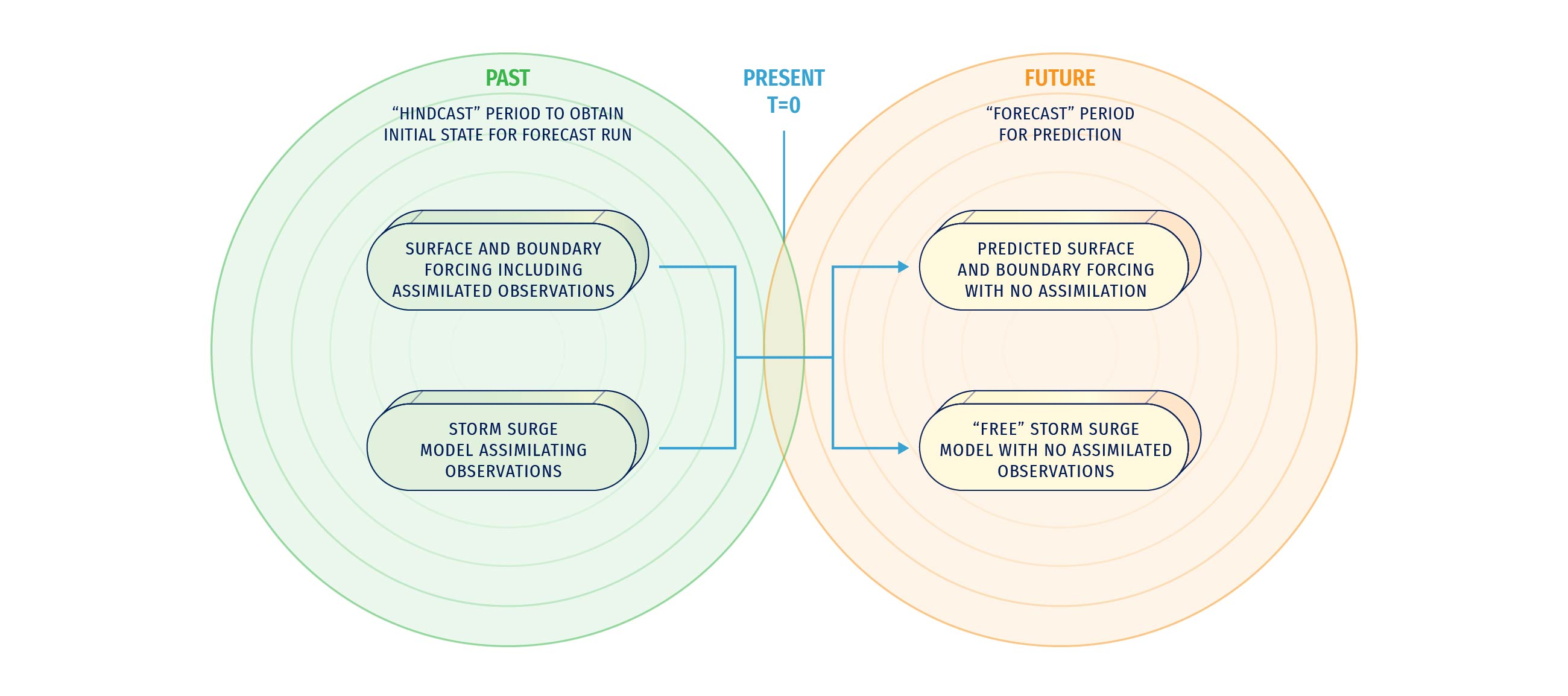
Figure 7.15. Illustration of two distinct stages of sequential data assimilation for forecasting storm surges.
This improved initial condition can be generated by running the model for some historical period up until today, including forcing with assimilated observations and potentially direct assimilation of sea surface height. This model run can effectively be seen as a continuous simulation with assimilative steps at some predefined frequency, for example every 6 hours. When a forecast is desired, the most recent state from this model can be taken and used as the initial condition. A forecast simulation is then done using no assimilation, as no observations are available in the future. This means that the atmospheric forcing used is also a forecast. Figure 7.15 illustrates this process.
There are several methods that have been used with success in storm surge modelling, including Optimal Interpolation (Gandin, 1966; Lorenc, 1981 and 1986; Daley, 1991), variational assimilation (Lorenc,1986), Kalman filters (Kalman,1960) and Ensemble Kalman Filters, (Evensen, 2004). In all methods, a key step is the estimation of spatial error covariances in both the model and the observations. This can be parametrically, as shown in the example in Figure 7.16, or by deriving covariances from an ensemble of model states. An example of the latter is described in Section 7.2.4.4.
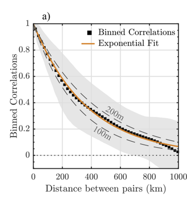
Figure 7.16. An example of correlation length scale estimation for assimilation of sea surface height into a barotropic storm surge model of the North Sea (Byrne et al. 2021). Such a length scale could be used to assimilate tide gauge observations.
Data assimilation has the potential to add significantly to the computation and time resources required, especially for ensemble systems. As noted, for real-time forecasting systems is vital that a balance is made between accuracy and speed, i.e. useful forecasts need to be delivered in a timely manner (Horsburgh et al., 2011).
7.2.4.4
Examples from real operational systems
The examples below are correct at the time of writing.
UKMO
The UK Met Office provides storm surge forecasting for the United Kingdom. Its 2D operational model does not currently assimilate any data into the model sea surface height. The atmospheric forcing used does include assimilated observations and comes from UKMO or the European Centre for Medium-Range Weather Forecasts (ECMWF) models, depending on the system. They also have more general operational 3D models that assimilate temperature, salinity and sea level anomaly, but the last is only done in deep water.
Rijkswaterstaat
Rijkswaterstaat provides storm surge forecasts for The Netherlands. Its system assimilates information from tide gauges around the Northwest European Shelf, especially in the North Sea (Verlaan et al., 2005; Zijl et al., 2015). They use a steadystate Kalman Filter (SSKF), which uses a stationary Kalman gain derived from an ensemble of states, such as might be used for the ensemble Kalman filter (EnKF). SSKF offers more computational efficiency than EnKF, and potentially a better representation of the error covariance than the standard Kalman Filter. Additional localization steps are also applied to the assimilation, to limit the distance from observations over which information is assimilated.
7.2.5
Ensemble modelling
Like any other forecasts, sea level predictions have an associated uncertainty. The threat to life and property of extreme sea level events makes estimation of this uncertainty and the generation of a range of possible water levels (probabilistic forecast) particularly important for risk managers and decision-makers. The error of a single forecast time series can be assessed by comparison with in-situ tide gauges at specific locations and grid points. However, uncertainty of the forecast and its dependence on the forcing, model characteristics, and set up is usually unknown.
Uncertainty of sea level forecasts depends on several factors and may contain errors in both the tide and the non-tidal residuals (storm surge) components. During a storm, the storm surge is mainly driven by the weather conditions at the sea surface. This is considered to be the dominant source of uncertainty in sea level forecasts and may change significantly depending on the meteorological conditions. For this reason, ensemble storm surge forecasts based on weather ensemble prediction systems (EPS) are the most common approach to generate probabilistic forecasts (forecast plus a confidence interval).
The weather is a chaotic system highly sensitive to the initial state (Lorenz, 1965) that can only be deterministically predicted for about 10 days. Therefore, the standard procedure for dealing with forecasts uncertainty, i.e. the combination of different model solutions or ensemble modelling, was initially applied to meteorological forecasts (Leith, 1974; Hamill et al., 2000). Conceptual background of ensembles is chaos theory; they are a valuable tool to deal with equations in which several nonlinear processes and interacting variables are present. This is the case of meteorological models but also of ocean models and, particularly, of tide and surge models. Hence, their application is today strongly recommended in oceanography.
An EPS is based on the combination of a set of forecasts with different controlled changes in the initial conditions, the model physics or the open boundary conditions (Palmer and Williams, 2010; Flowerdew et al., 2010). All these modifications are designed to represent the uncertainties in the knowledge of the weather state. For example, different initial conditions allow to include those perturbations that grow most rapidly in time, in a context where slight changes to the initial conditions may lead to significantly different forecasts (Buizza and Palmer, 1995). Slight modifications of the set of equations (including different values in the parameterization constants representing different processes) also provide estimation of model uncertainties contributing to the forecast error.
Deviation of wind and sea level pressure fields from their actual evolution will determine a corresponding deviation on the predicted sea level. Therefore, their uncertainty derived from weather EPS will cause an uncertainty in the evolution of the sea level, linked to the meteorological forcing and affecting mainly the storm surge component. If different weather predictions are used to drive different sea level simulations, the probability distribution function of the forecast sea level values allows estimating the uncertainty of the sea level forecast and the probability of exceeding a given sea level threshold.
The ECMWF EPS has been operational since 1992 (Molteni et al., 1996). It was first applied to storm surge operational forecasts in the North Sea by Flowerdew et al. (2010 and 2013), who provided skilled probabilistic forecasts of sea level and showed that ensemble spread was a reliable indicator of uncertainty during large surge events.
Storm surge ensemble predictions have been used to forecast sea level in Venice by Mel and Lionello (2014a). They used a 50 members ensemble to simulate 10 events showing that EPS slightly increases the accuracy of the prediction with respect to the deterministic forecast, and that the probability distribution of maximum sea level produced by the EPS is acceptably realistic. They also showed that the storm surge peaks correspond to maxima of uncertainty and that the uncertainty of such maxima increases linearly with the forecast range. The same procedure was used by Mel and Lionello (2014b) for the simulation of the operational forecast practice for a three-month period (fall 2010). It revealed that uncertainty for short and long lead times of the forecast is mainly caused by the uncertainty of the initial condition and of the meteorological forcing, respectively. The probability forecast based on this ensemble technique has a clear skill in predicting the actual probability distribution of sea level. A computationally cheap alternative, called ensemble dressing method, has been proposed by Mel and Lionello (2016). It replaces the explicit computation of uncertainty by ensemble forecast with an empirical estimate. Instead of performing multiple forecasts, the procedure “dresses” the forecast of sea level with an error distribution form, which includes, on one hand, a dependence of the uncertainty on surge level and lead time and, on the other hand, of the uncertainty of the meteorological forcing. This computationally cheap alternative also provides acceptably realistic results.
Apart from the meteorological input, other sources of error on sea level forecasts can be attributed to the ocean model characteristics and/or to the setup of the system: bathymetry, spatial resolution, model domain, tidal forcing, temporal resolution of the meteorological input, barotropic or baroclinic models, ocean open boundary conditions, etc. Currently, sea level variations on timescales of hours/days are operationally forecasted through different barotropic and baroclinic models, sometimes over the same area. Therefore, another option is the combination of existing operational models with different characteristics, forcings and even physics (multi-model forecast).
A multi-model storm surge forecast was first implemented by Deltares (an independent Dutch institute) in 2008, combining existing operational storm surge forecasts from different countries in the North Sea. The system included the use of the Bayesian Model Average (BMA) statistical technique for validation of the different members and generation of a combined improved prediction, with a confidence interval (Beckers et al., 2008). In the same year, this methodology was tested for the Spanish coast by Puertos del Estado (Spain) (Pérez et al., 2012), combining the output of Nivmar (Álvarez-Fanjul et al., 2001), an existing storm surge forecasting system, with circulation (baroclinic) models already operating in the region. Nowadays, at Puertos del Estado is operational a multi-model surge forecast named ENSURF that combines Nivmar with two Copernicus Marine Service regional operational models, IBI-MFC (Sotillo et al., 2015) and MedFS (Clementi et al., 2021).
The BMA technique requires near-real time access to tide gauge data and automatic quality control of this data (as required by the Nivmar system as well), and specific data tailoring of model outputs. It is applied to the surge or non-tidal residual component of sea level because this can be approximated by a normal distribution (which is not the case for total sea level including tides, especially for strong semidiurnal regimes). So, observations from tide gauges and model data for those models providing total sea level must be previously decided. This could be considered a limitation but, in practice, it is the best way of optimising the final total sea level forecast by using the tidal component obtained from historical tide gauge observations at each site. ENSURF is also a valuable operational validation tool that allows a detailed assessment of the skills of different models to forecast coastal sea levels. A first deterministic forecast is provided by the old Nivmar solution early in the morning every day and, when later the Copernicus Marine Service forecasts become available, they are integrated with the tide gauge data and, by means of the BMA technique, a probabilistic forecast band is generated for each harbour (Pérez-González et al., 2017, Pérez-Gómez et al., 2019) (Figure 7.17).
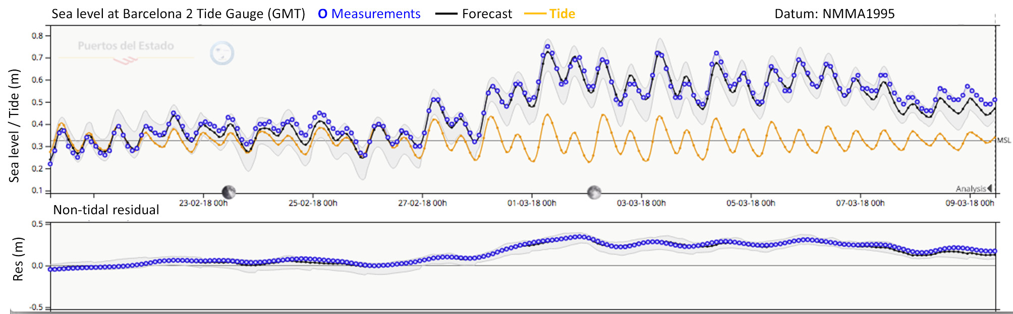
Figure 7.17. Example of sea level probabilistic forecast generated by the multi-model ENSURF for the Barcelona harbour, validated against Barcelona tide gauge (hourly data). Top panel: total sea level; bottom panel: surge component. Blue: tide gauge data; orange: tide prediction; black: BMA forecast; grey: BMA confidence interval.
Generally, use of the probabilistic methodology improves the forecast and gives significant added value to existing operational systems, as there is no single model that outperforms at all tidal stations and synoptic conditions. However, further work must be done with the BMA technique to predict the storm peaks which, in some weather conditions, are better captured by single systems.
A multi-model ensemble forecasting system has been recently developed for the Adriatic Sea combining 10 models predicting sea level height (either storm surge or total water level) and 9 predicting waves characteristics (Ferrarin et al., 2020). Other examples of this technique can be found in New York (Di Liberto et al., 2011) and the North Sea (Siek and Solomatine, 2011).
7.2.6
Validation strategies
Storm surge models have been traditionally validated with time series of coastal sea level measured by tide gauges. These data allow assessing the skills of the model to reproduce observed water heights at specific points along the coast. Note the advantages this application presents with respect to sea level data from satellite altimetry, less reliable along the coastal strip and with a lower temporal resolution. Fortunately, there are hundreds of tide gauges around the world that become a very valuable and reliable dataset for storm surge validation (Muis et al., 2016 and 2020, Fernández-Montblanc et al., 2020). In some cases, these stations provide ancillary meteorological data, such as wind and atmospheric pressure, which can also be used to validate the model meteorological forcing. In addition, tide gauges transmit data in near-real time that can be integrated in an operational validation of the forecasting system (Álvarez-Fanjul et al., 2001).
In most cases, the forecast will provide the tide and storm surge signals (hourly to daily timescales), usually dominant at the tide gauge records, but will not be able to reproduce higher-frequency sea level oscillations such as infragravity waves, seiches or meteotsunamis, with periods of the order of a few minutes. It is important to define which observed “sea level” product will best fit the validation purpose, according to the physical processes included in the system. The most adequate standard product for existing operational storm surge forecasting systems are filtered hourly values from tide gauges. As new models include additional processes (e.g. fully coupled models including wave effects), higher resolution bathymetries, and forcing fields, the use of lower temporal sampling data will become more important and the validation process more challenging.
Normally, the model output at the grid point closer to the tide gauge is selected. However, the validation results will depend on the resolution and quality of the bathymetry data, as well as on the location of the tide gauge: if it is in an open site or inside a harbour or bay with important local effects, it may not be resolved by the model.
A careful validation of both tide and surge components should be performed to verify not only the final total sea level forecast, but also the quality of the tidal signal in the model, which can be an important source of error especially on shallow waters with high tidal range. For these reasons, model and tide gauge data must be de-tided, applying a harmonic analysis to both time series, as well as computing the tide prediction for the analysed period, and the surge or non-tidal residual after tide subtraction. The performance assessment can then be made in terms of comparison of the harmonic constants (amplitude and phase) from model and observations, and in terms of model data time series comparison of tide, surge and total sea level.
It is important to mention that sea levels measured by the tide gauge will be related to a local, regional or national datum. The model forecast is theoretically referred to mean sea level, though this mean sea level may be affected by the model setup implementation, domain, etc. Therefore, the mean should be subtracted from both time series at each location before comparison.
Metrics for time series validation can be found at Section 4.5.1. Most of these metrics describe the overall performance of the model for a time period of several days (the storm duration), months or years. However, they do not reflect the predictive skill for extreme surge events. This can be better evaluated, for example, in terms of the differences in the highest percentiles (e.g.: 95th, 99th percentiles) or the maximum observed and modelled value. For validation of long time series (multi-decadal hindcasts), it is possible to use annual maxima, annual percentiles, and extreme sea levels for specific return periods, obtained through extreme sea level analysis (Muis et al., 2020).
Taylor diagrams can be used to graphically indicate the performance of different competing models or solutions, providing information of the Pearson correlation coefficient, the standard deviation and the RMSE at each tide gauge.
Progressively, the storm surge models will consider inundation, and additional validation of the flooding extent will be required. This is less straightforward and requires other types of data, such as locations of flooded points, marks left by the water or reports about the flood chronology (Le Roy et al., 2015). This information is commonly available after the event for a delayed mode validation; e.g. for validation of inundation, Loftis et al. (2017) used crowdsourced GPS data and maps of flooded areas obtained by drones.
7.2.7
Outputs
The main outputs of storm surge models are: time series output, maximum elevation field output (extreme values at every time step for water surface elevation), ensemble forecast elevation field output, animation output.
7.2.7.1
Time series outputs
The time series output is usually plotted in a two-dimensional rectangular coordinate system, the abscissa is time and the ordinate is water level. The time series output of storm surge models are the water level changes at a certain location. In order to facilitate the comparison between the results of simulations and the observation data, multiple result curves can be plotted in the same coordinate system.
Generally, the results of storm surge models (without tide) can be directly used for plotting time series diagrams, but sometimes attention should be paid to the change of the total water level at a certain point. Therefore, there is a way to output the total water level, that is the results of the storm surge model without astronomical tide directly superimposed on the astronomical tide from harmonic analysis, obtaining in this way the time series results of the total water level. Figures 7.18 and 7.19 show examples of time series model storm surge result and storm surge superimpose on harmonic analysis tide.
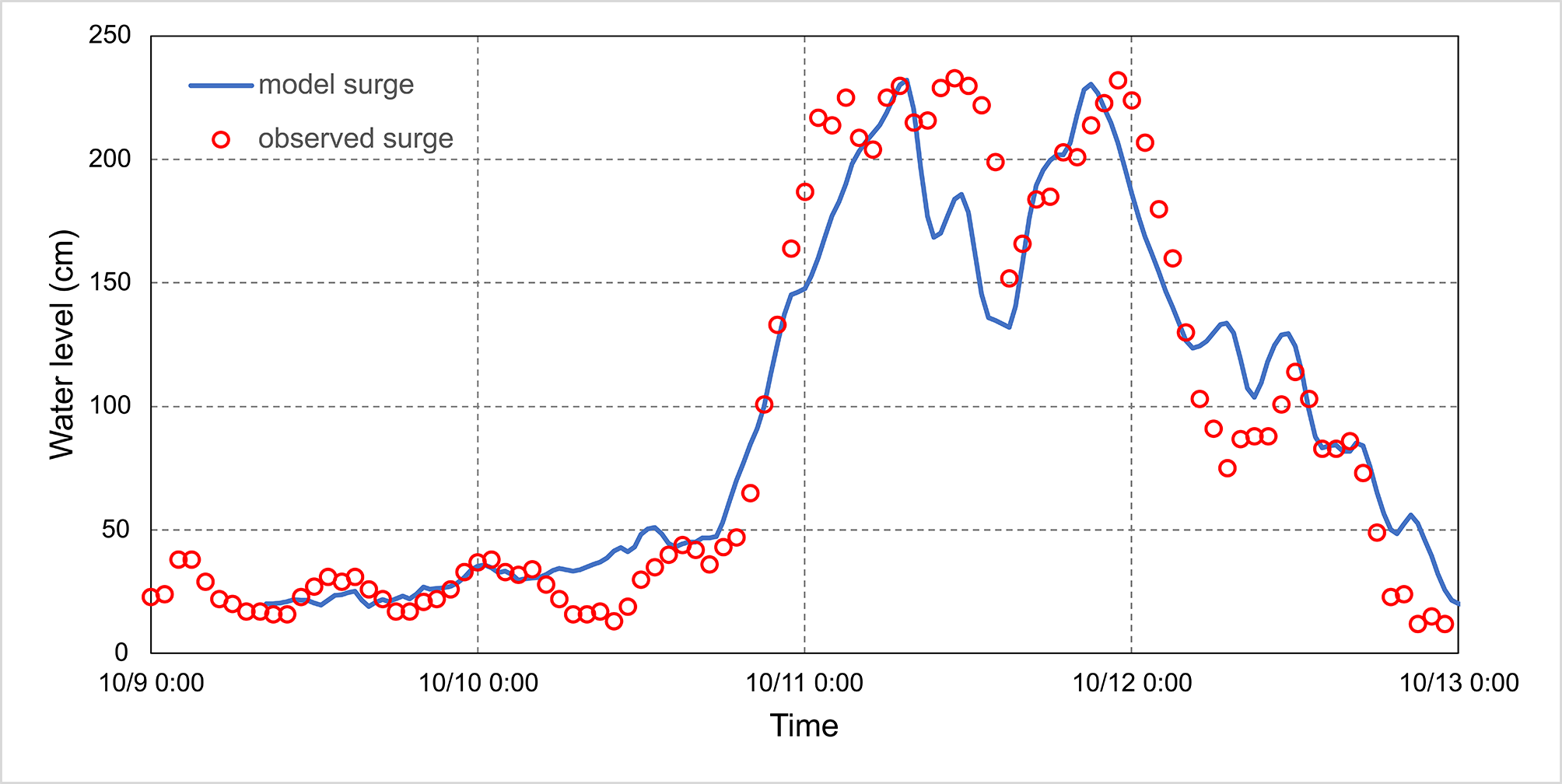
Figure 7.18. Time series model storm surge result (blue line) and observed storm surge (red circle).
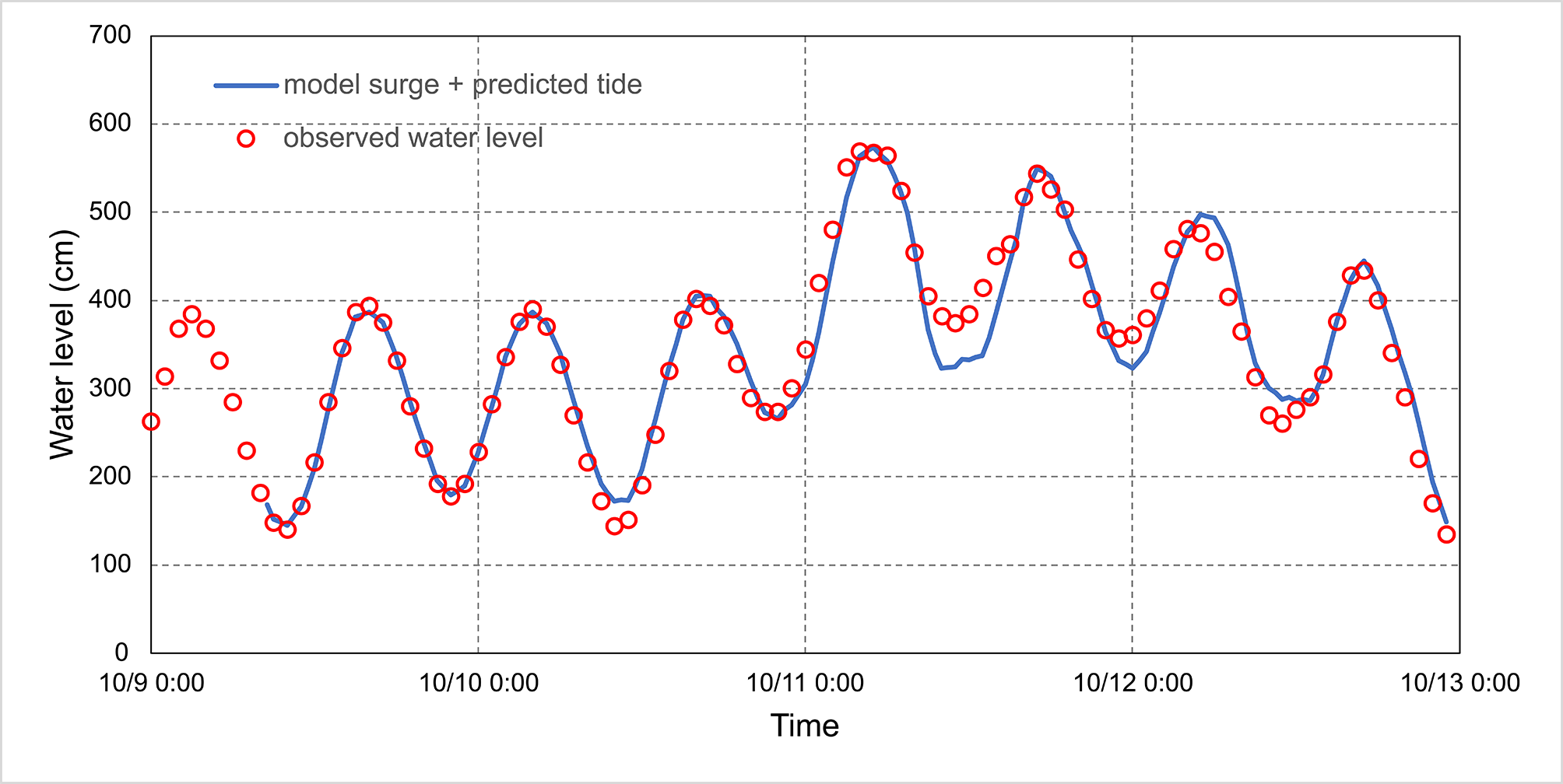
Figure 7.19. Time series model storm surge result superimposed on predicted tide (blue line) and observed water level (red circle).
7.2.7.2
Maximum elevation field
Among the output methods of storm surge models, there is an output form called maximum elevation field. This kind of field output is not the water level field at a certain time, but extracts the highest water level value of each grid point in the calculation process to form the maximum elevation field. The maximum water level field can be used to grasp the distribution of the maximum water level during a Typhoon and to identify the more severely affected areas along the coast. Figure 7.20 shows the maximum storm surge field during 2019 Typhoon Mitag (1918).
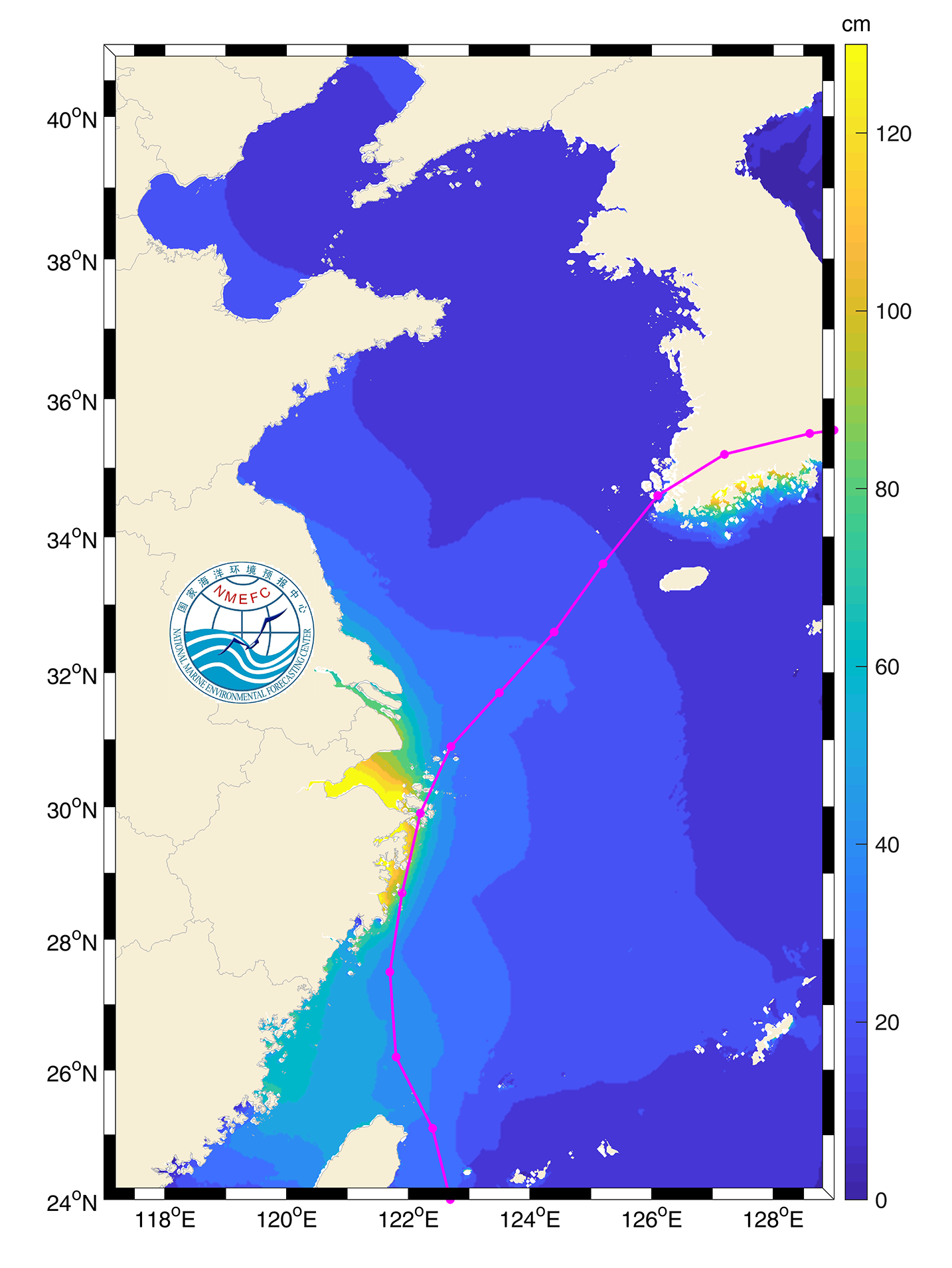
Figure 7.20. The maximum storm surge field during 2019 Typhoon Mitag (1918).
7.2.7.3
Ensemble forecast field
The storm surge ensemble forecast usually uses the respective meteorological forcing fields of the ensemble members to calculate the storm surge separately. The output of ensemble forecast fields mainly includes the following forms: (a) ensemble mean field; (b) probability field; and (c) postage stamp maps.
a. Ensemble mean storm surge field
In order to obtain a definite forecast result, it is necessary to synthesise the respective results of the ensemble members. It is generally used to assign different weights to the results of each member and to superimpose the results of all members, i.e. the weighted average method (Wang et al., 2010). The superimposed result is output in the form of the elevation field, and the ensemble forecast field is obtained as result.
The track map of Typhoon Mitag can be seen in Figure 7.21. The storm surge results of the subjective typhoon forecast track, fast track, slow track, left track, and right track are used to synthesise the ensemble forecast water level field applying the weighted average method (Figure 7.22). In this example, the weight of the storm surge result of the subjective forecast typhoon track is 60%, while the weight of the storm surge result of the other tracks are all 10%.

Figure 7.21. Track map of Typhoon Mitag. Red line: middle track; black line: fast track; cyan line: slow track; magenta line: left track; blue line: right track.
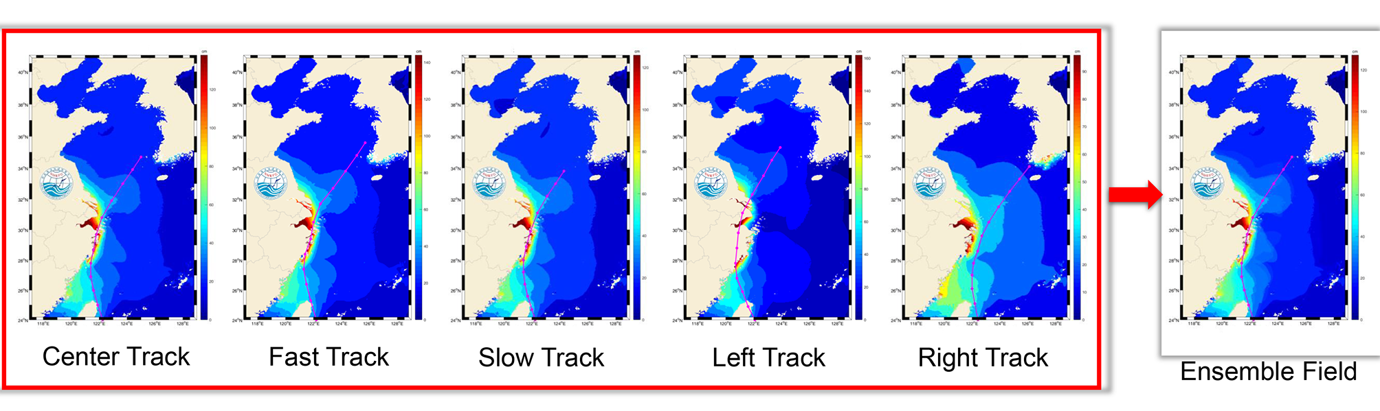
Figure 7.22. Synthesis of ensemble forecast water level field.
b. Probability storm surge field
The typhoon ensemble forecasting tracks for storm surge numerical simulation can describe the surge field under different typhoon track scenarios. By equitably assigning weights to different track results, the probability field distributions under different extreme values of storm surges can be clearly displayed, and the intensity probability of coastal storm surges can be more intuitively presented (Liu et al., 2020). Figures from 7.23 to 7.25 show the probability distribution of forecast storm surge over 0.5m, 1.0m and 2.0m of Typhoon Mitag.
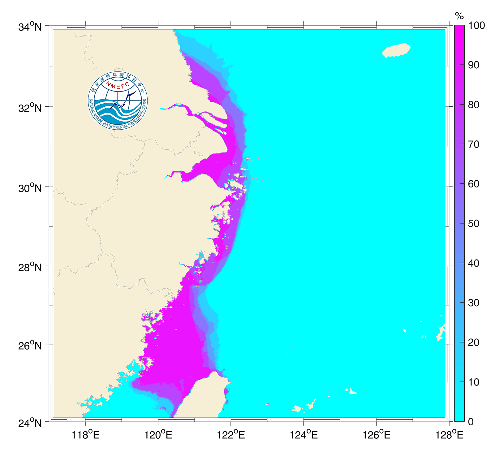
Figure 7.23. Distribution of probability forecasting of storm surge over 0.5m.
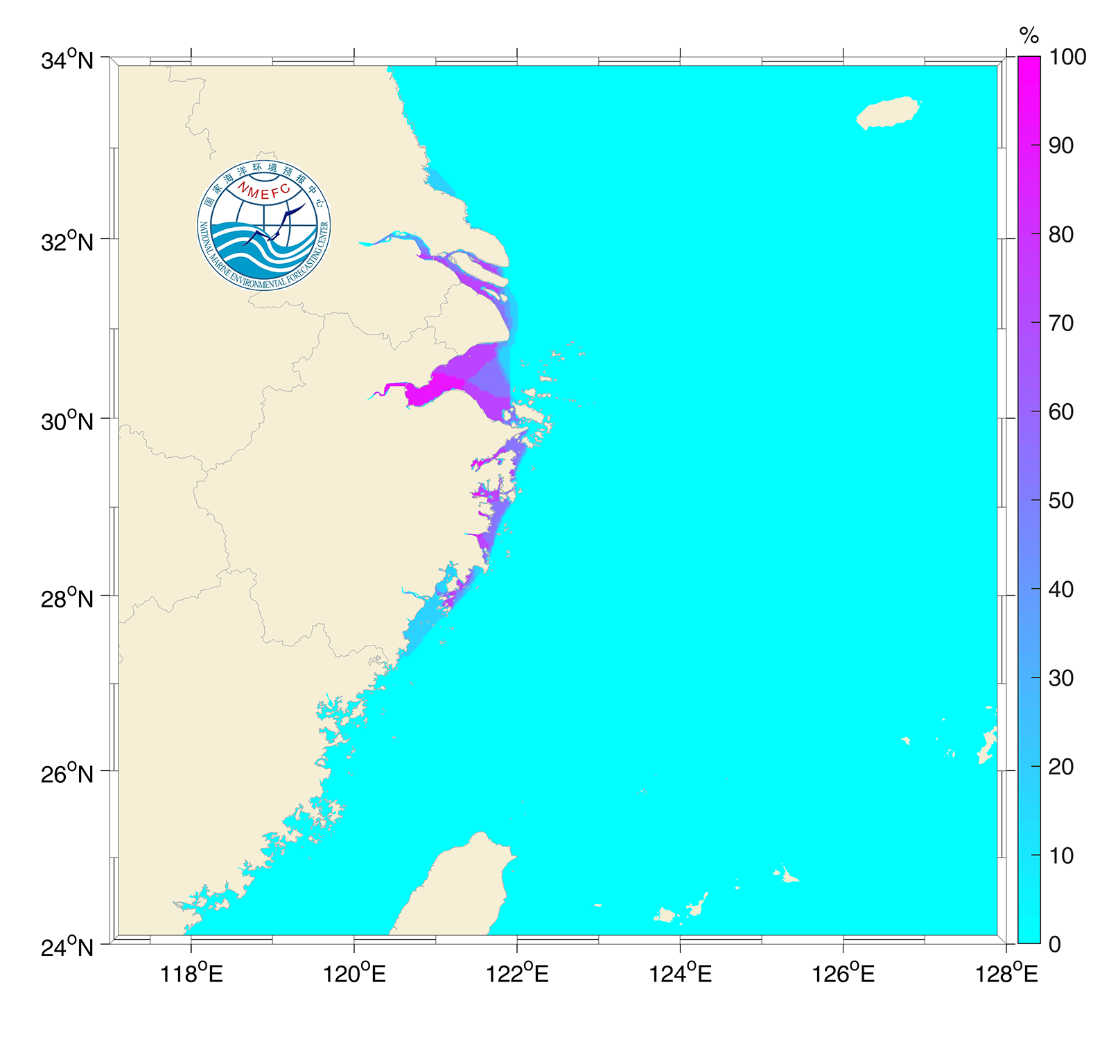
Figure 7.24. Distribution of probability forecasting of storm surge over 1.0m.
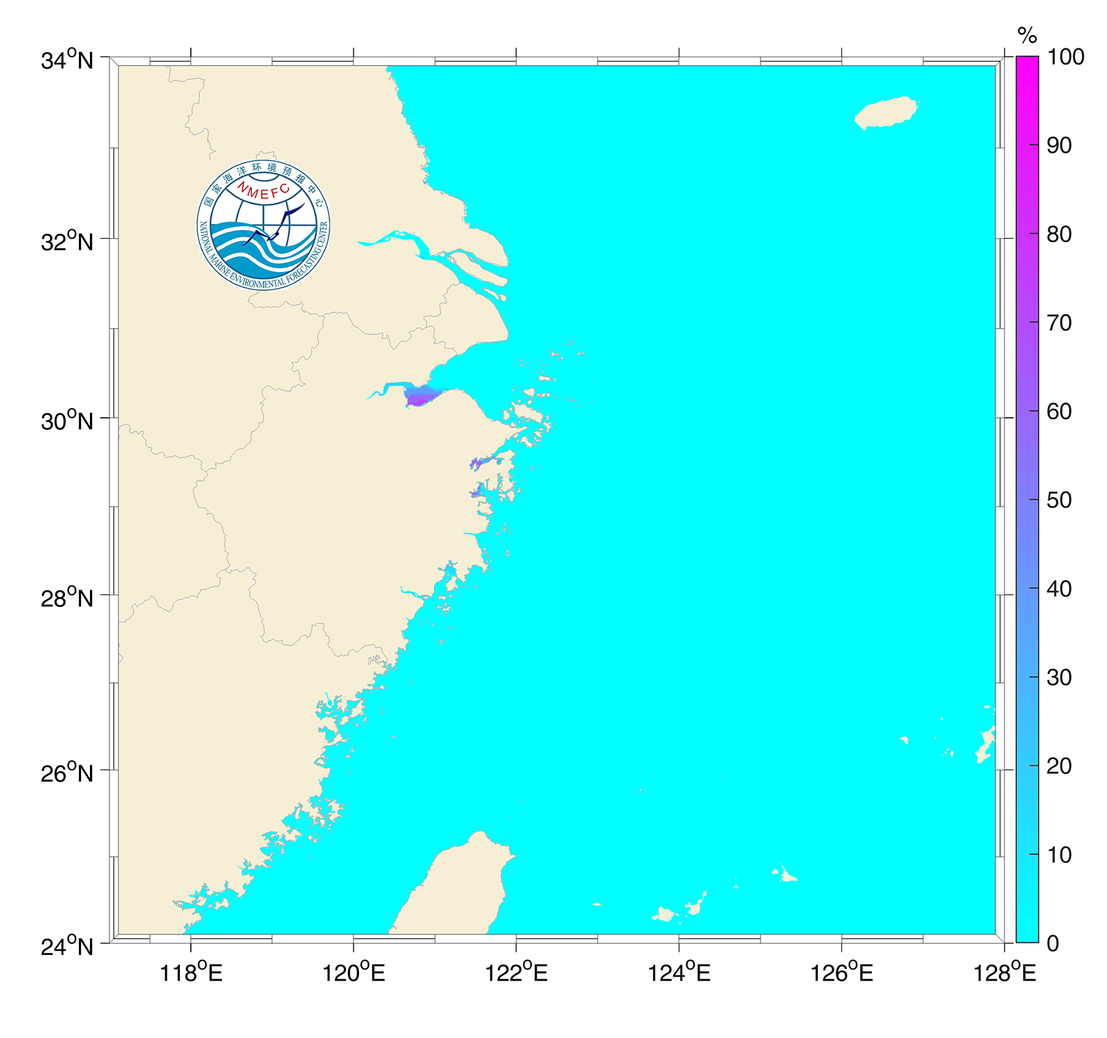
Figure 7.25. Distribution of probability forecasting of storm surge over 2.0m.
c. Postage stamp maps
A postage stamp map is a set of small storm surge maps drawn by the results of the individual members (Figure 7.26). Forecasters can learn about the possible situation of each ensemble member through the postage stamp map, thereby estimating the magnitude of the maximum storm surge and the range of impact. (WMO, 2012).
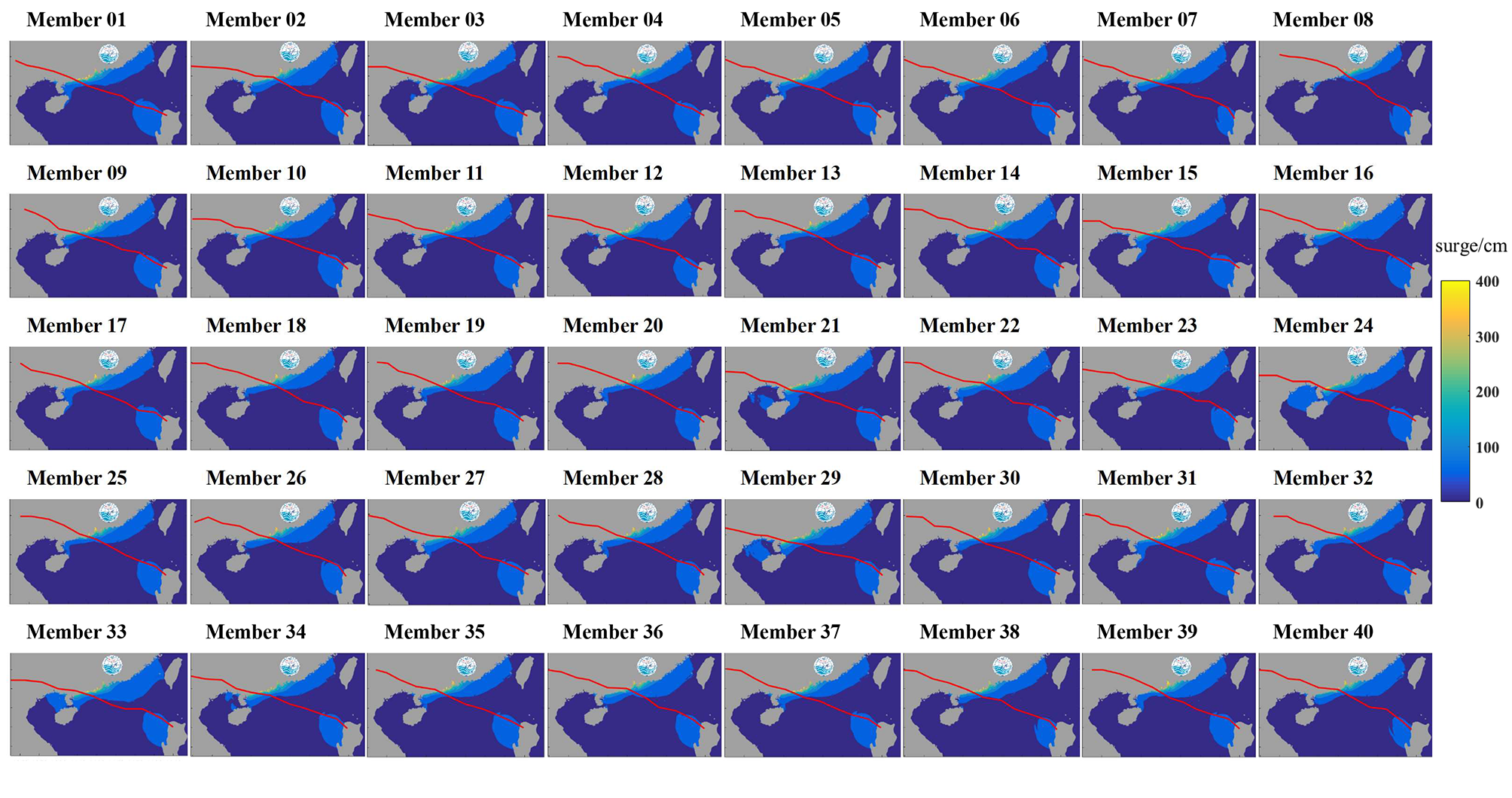
Figure 7.26. Postage stamp map of storm surge field of Typhoon Mangkhut.
7.2.7.4
Animation output
The output of the water level field is very helpful for grasping the distribution of the storm surge process over a whole region. The output of the storm surge water level field is the elevation value of all grid points at a certain time. The elevation field figure at each moment is taken as a frame of the animation, and all the frames are connected to form the elevation field animation (Figure 7.27). The elevation field animation can intuitively reflect the changes in the water level of the entire area during the impact of the storm surge.
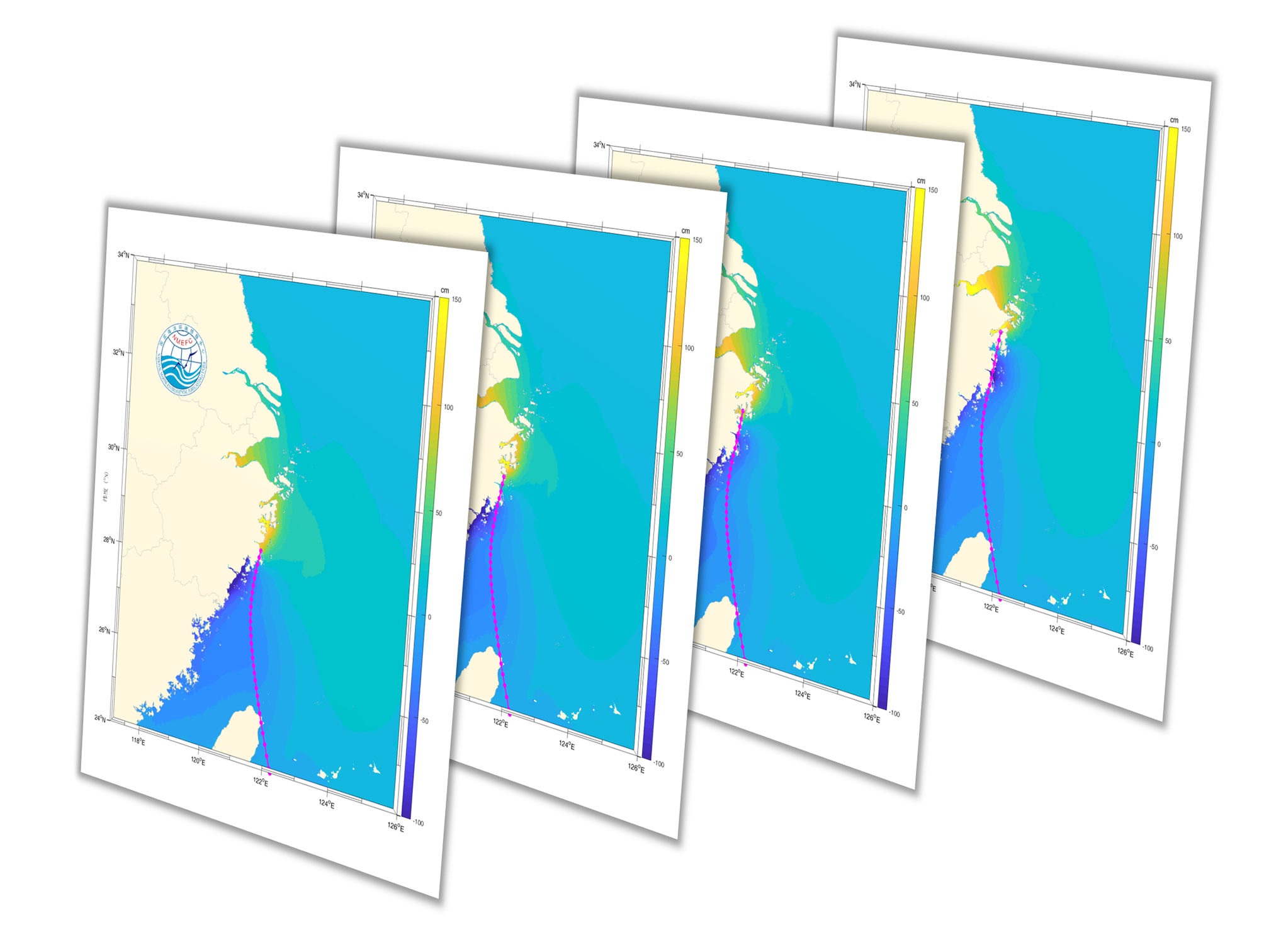
Figure 7.27. Synthesis of elevation field animation.
7.2.8
Existing operational storm surge forecasting systems
After decades of development of storm surge numerical models, many countries have established their own operational storm surge forecasting models. For example, in the United States a storm surge forecasting system is operating through the SLOSH model, in which the wind field is established based on the cyclone path, maximum wind speed radius, storm centre, and environmental pressure difference; it provides operational forecast products and storm surge inundation guidance products (Jarvinen and Lawrence,1985). China established ver3.0 of the PMOST forecasting system, which is based on a depth-averaged two-dimensional shallow water equation in the vector invariant form, and uses a SCVTs grid. It can enhance the resolution in key areas and fit the coastline. The system is able to couple astronomical tides and simulate flooding processes. With the GPU acceleration technology, the efficiency of storm surge simulation along the coast of China can reach 60 sec/day. The system can also perform ensemble forecasts based on multiple typhoon events and storm surge probability forecasting. The Indian Institute of Technology storm surge model was developed in the 1980s and applied to storm surge forecasts in the Indian Ocean and the Arabian Sea. It uses rectangular Cartesian coordinates and separates land and water during calculations. It has been applied throughout the north Indian Ocean (Dube et al., 1984, Dube et al., 1985).
The two-dimensional storm surge model developed by the Japan Meteorological Agency also uses rectangular coordinates (Hasegawa et al., 2015). In the numerical calculation, the water and land are separated with the flexible mesh, i.e. fine grid is used in shallow water and coarse grid is used in deep water. The system can also provide ensemble forecasting products. In the mid-1980s, the Netherlands developed a numerical fluid dynamics model called the DCSM, which uses a depth integrated shallow water equation. The driving force of the model is provided by a high-resolution regional meteorological model. In the early 1990s, the Kalman filtering method was used in DCSM to assimilate the water level (Verlaan et al., 2005; de Vries, 2009). The UKMO developed the storm surge forecasting model CS3X, which is a tide-storm surge model. In this operational storm surge forecasting system, the interaction of tide and storm surge is considered. In recent years, a storm surge ensemble forecasting has been developed in this system (Flowerdew et al., 2013). A storm surge model covering the French overseas territories has been operated since the 1990s by Meteo-France (Daniel et al., 2009); it was established based on the spherical nonlinear shallow water equation. In order to solve the problem of the shore boundary, the C-grid difference format was adopted, with meteorological forcing provided by the Holland model (see Section 7.2.2.3). Table 7.2 provides a list and features of storm surge forecasting systems currently operating in various countries.
| Model | Area | Type | Grid | Country |
|---|---|---|---|---|
| HAMSOM, Nivmar | Mediterranean Sea and Iberian Peninsula | Vertically integrated barotropic | 10 minutes | Spain |
| Mike 21 preoperational 3-D 2-D finite element MOG2D | North Sea, Baltic Sea | 2-D hydrodynamic | Finite difference 9 nmi, 3 nmi, 1 nmi, 1/3 nmi | Denmark |
| Coupled ice–ocean NPAC | Grand Banks, Newfoundland, Labrador NE Pacific, 120°W–160°W, 40°N–62°N | 3-D circulation based on the Princeton Ocean Model | Approximately 20 km x 20 km Finite difference curvilinear C-grid 1/8 degree | Canada |
| Mike 21 preoperational 3-D 2-D finite element MOG2D | North Sea, Baltic Sea | 2-D hydrodynamic | Finite difference 9 nmi, 3 nmi, 1 nmi, 1/3 nmi | Denmark |
| JMA Storm Surge | 23.5°N–46.5°N, 122.5°E–146.5°E | 2-D linearized shallow water | Staggered Arakawa C-grid. 1 minute latitude/longitude | Japan |
| KMA Storm Surge | 20°N–50°N, 115°E–150°E | 2-D barotropic surge and tidal current based on the Princeton Ocean Model | Approximately 8 km x 8 km, finite difference curvilinear C-grid 1/12 degree | Republic of Korea |
| NIVELMAR | Portuguese mainland coastal | Shallow water | 1 minute latitude x 1 minute longitude | Portugal |
| SMARA storm surge | Shelf sea 32°S–55°S, 51°W–70°W. Rio de la Plata | 2-D depth-averaged | Geographical Arakawa C-grid, 1/3 degree latitude x 1/3 degree longitude 1/20 degree latitude x 1/20 degree longitude | Argentina |
BSH circulation (BSHcmod) BSH surge (BSHsmod) | North-east Atlantic, North Sea, Baltic | 3-D hydrostatic circulation 2-D barotropic surge | Regional spherical, North Sea, Baltic 6 nmi, German Bight Western Baltic, 1 nmi, surge North Sea, 6 nmi, north-east Atlantic 24 nmi | Germany |
| Caspian Storm Surge | Caspian Sea 36°N–48.5°N, 45°E–58°E North Caspian Sea 44.2°N–48°N, 46.5°E–55.1°E | 2-D hydrodynamic, based on MIKE 21 (DHI Water & Environment) | 10 km x 2 km | Kazakhstan |
| HIROMB/NOAA | North-east Atlantic, Baltic | 3-D baroclinic | C-grid, 24 nmi | Sweden |
| WAQUA-inSimona/DCSM98 | Continental shelf 48°N–62°N, 12°E–13°E | 2-D shallow water, ADI method, Kalman filter data assimilation | 1/8 degree longitude x 1/12 degree latitude | Netherlands |
| Derived from MOTHY oil spill drifts model | Near-Europe Atlantic (Bay of Biscay, Channel and North Sea) 8.5°E–10°E, 43°N–59°N West Mediterranean basin (from the Strait of Gibraltar to Sicily) Restricted area in overseas departments and territories | Shallow-water equations | Arakawa C-grid 5’ of latitude x 5’ of longitude Finer meshes | France |
| SLOSH | Sea area south of Hong Kong within 130 km | Finite difference | Polar, 1 km near to 7 km, South China Sea | Hong Kong, China |
| Short-term sea-level and current forecast | Caspian Sea and near-shore lowlying zones | 3-D hydrodynamic baroclinic | 3 nmi horizontal, 19 levels | Russian Federation |
| IIT–Delhi, IIT–Chennai, NIOT–Chennai | East and west coasts of India and high-resolution areas | Non-linear, finite element, explicit finite element | For inundation model average spacing of 12.8 km offshore direction and 18.42 km along shore | India |
| CS3 tide surge | North-west European shelf waters | Finite difference, vertically averaged | C-grid 12 km, nested finer resolution | United Kingdom |
| SLOSH | Atlantic and gulf coasts | 2-D depth integrated | 625 meters | United States |
| PMOST 3.0 | China sea 10°N~45°N, 105°E~140°E | 2-D depth-averaged barotropic | SCVTs unstructured grid, 10km at boundary and 500m along shoreline | People's Republic of China |
Table 7.2. List and features of operational storm surge forecast models.
References
Álvarez-Fanjul, E., Perez Gomez, B., Sanchez Arevalo, I.R. (2001). Nivmar: A storm surge forecasting system for Spanish Waters. Scientia Marina, 65(S1), https://doi.org/10.3989/scimar.2001.65s1145
Beckers J. V. L., Sprokkereef, E., and Roscoe, K. L. (2008). Use of Bayesian model averaging to determine uncertainties in river discharge and water level forecasts, Proceeding of “4th International Symposium on Flood Defence: Managing Flood Risk, Reliability and Vulnerability”, Toronto, Ontario, Canada, 6–8 May, 2008.
Bjerknes, V. (1921). On the dynamics of the circular vortex with applications to the atmosphere and atmospheric vortex and wave motions. Quarterly Journal of the Royal Meteorological Society, 48(204), 375-376. https://doi.org/https://doi.org/10.1002/qj.49704820414
Buizza, R., and Palmer, T.N. (1995). The Singular-Vector Structure of the Atmospheric Global Circulation. Journal of the Atmospheric Sciences, 52(9), 1434-1456, https://doi.org/10.1175/1520-0469(1995)052<1434:TSVSOT>2.0.CO;2
Byrne, N. J. (2017). Deterministic models of Southern Hemisphere circulation variability. Ph.D. thesis, University of Reading, 105 pp.
Byrne, D., Horsburgh, K., and Williams, J. (2021). Variational data assimilation of sea surface height into a regional storm surge model: Benefits and limitations. Journal of Operational Oceanography, 1-14, https://doi.org/10.1080/1755876X.2021.1884405
Clementi, E., Aydogdu, A., Goglio, A. C., Pistoia, J., Escudier, R., Drudi, M., Grandi, A., Mariani, A., Lyubartsev, V., Lecci, R., Cretí, S., Coppini, G., Masina, S., and Pinardi, N. (2021). Mediterranean Sea Physical Analysis and Forecast (CMEMS MED-Currents, EAS6 system) (Version 1) set. Copernicus Monitoring Environment Marine Service (CMEMS), https://doi.org/10.25423/CMCC/medsea_analysisforecast_PHY_006_013_EAS6
Daley, R. (1991). Atmospheric Data Analysis. Cambridge University Press: Cambridge, UK
Daniel, P., Haie, B., and Aubail, X. (2009). Operational Forecasting of Tropical Cyclones Storm Surges at Meteo-France. Marine Geodesy, 32(2), 233-242. https://doi.org/10.1080/01490410902869649
de Vries, H. (2009). Probability Forecasts for Water Levels at the Coast of The Netherlands. Marine Geodesy, 32(2), 100-107, https://doi.org/10.1080/01490410902869185
Di Liberto, T., and Colle, B.A. (2011). Verification of a Multimodel Storm Surge Ensemble around New York City and Long Island for the Cool Season. Weather and Forecasting, 26, 922-939.
Doodson, A. T. (1929). Report on Thames Floods. Geophysical Memoirs, Great Britain Meteorological Office, 5(47), 1-26.
Doodson, A. T. (1956). Tides and storm surges in a long uniform gulf. Proceedings of the Royal Society of London. Series A. Mathematical and Physical Sciences, 237(1210), 325-343.
Dube, S. K., Sinha, P. C., Rao, A. D., and Rao, G. S. (1985). Numerical modelling of storm surges in the Arabian Sea. Applied Mathematical Modelling, 9(4), 289-294, https://doi.org/https://doi.org/10.1016/0307-904X(85)90067-8
Dube, S. K., Sinha, P. C., and Roy, G. D. (1984). Numerical simulation of storm surges induced by tropical storms impinging on the Bangladesh coast. Coastal Engineering Proceedings, 1(19), https://doi.org/10.9753/icce.v19.13
Egbert, G. D., Bennett, A. F., and Foreman, M. G. G. (1994). TOPEX/POSEIDON tides estimated using a global inverse model. Journal of Geophysical Research: Oceans, 99(C12), 24821-24852, https://doi.org/10.1029/94JC01894
Egbert, G. D., and Erofeeva, S. Y. (2002). Efficient Inverse Modeling of Barotropic Ocean Tides. Journal of Atmospheric and Oceanic Technology, 19(2), 183-204, https://doi.org/10.1175/1520-0426(2002)019<0183:Eimobo>2.0.Co;2
Evensem, G. (2004). Sampling strategies and square root analysis schemes for the EnKF. Ocean Dynamics, 54, 539-560, https://doi.org/10.1007/s10236-004-0099-2
Fernández-Montblanc, T., Vousdoukas, M.I., Mentaschi, L., Ciavola, P. (2020). A Pan-European high resolution storm surge hindcast. Environment International, 135, 105367, https://doi.org/10.1016/j.envint.2019.105367
Ferrarin, C., Valentini, A., Vodopivec, M., Karic, D., Massaro, G., Bajo, M., De Pascalis, F., Fadini, A., Ghezzo, M., Menegon, S., Bressan, L., Unguendoli, S., Fettich, A., Jerman, J., Licer, M., Fustar, L., Papa, A.. Carraro, E. (2020). Integrated sea storm management strategy: the 29 October 2018 event in the Adriatic Sea. Natural Hazards and Earth System Sciences, 20, 73-93, https://doi.org/10.5194/nhess-20-73-2020
Flowerdew, J., Horsburgh, K., Wilson, C., and Mylne, K. (2010). Development and evaluation of an ensemble forecasting system for coastal storm surges. Quarterly Journal of the Royal Meteorological Society, 136(651), 1444-1456, https://doi.org/10.1002/qj.648
Flowerdew, J., Mylne, K., Jones, C., and Titley, H. (2013). Extending the forecast range of the UK storm surge ensemble. Quarterly Journal of the Royal Meteorological Society, 139(670), 184-197, https://doi.org/10.1002/qj.1950
Fujita, T. (1952). Pressure distribution within typhoon. Geophysical Magazine, 23, 437-451.
Gandin, L.S. (1963). Objective analysis of meteorological fields. Translated from Russian.
Hamill, T. M. , Snyder, C., and Morss, R.E. (2000). A comparison of probabilistic forecasts from bred, singular vector, and perturbed observation ensembles. Monthly Weather Review, 128(6), 1835-1851, https://doi.org/10.1175/1520-0493(2000)128<1835:ACOPFF>2.0.CO;2
Harris, D.L. (1957). The Effect of a Moving Pressure Disturbance on the Water Level in a Lake. In: “Interaction of Sea and Atmosphere”. Meteorological Monographs, vol 2. American Meteorological Society, Boston, MA. https://doi.org/10.1007/978-1-940033-15-0_4
Hasegawa, H., Kohno, N., and Itoh, M. (2015). Development of Storm Surge Model in Japan Meteorological Agency. Available at http://www.waveworkshop.org/14thWaves/Papers/JCOMM_2015_J4.pdf
Heemink, A.W. (1986). Storm surge prediction using Kalman filtering. Dissertation TU Twente, Hydraulic Engineering Reports. Available at http://resolver.tudelft.nl/uuid:8a7c65f5-f8f5-4033-b796-adaef2eb39a7
Hersbach, H. Bell, B., Berrisford, P., Hirahara, S., Horányi, A., Muñoz-Sabater, J., Nicolas, J., Peubey, C., Radu, R., Schepers, D., Simmons, A., Soci, C., Abdalla, S., Abellan, X., Balsamo, G., Bechtold, P., Biavati, G., Bidlot, J., Bonavita, M., De Chiara, G., Dahlgren, P., Dee, D., Diamantakis, M., Dragani, R., Flemming, J., Forbes, R., Fuentes, M., Geer, A., Haimberger, L., Healy, S., Hogan, R.J., Hólm, E., Janisková, M., Keeley, S., Laloyaux, P., Lopez, P., Lupu, C., Radnoti, G., de Rosnay, P., Rozum, I., Vamborg, F., Villaume, S., Thépaut Hersbach, J.N. (2020). The ERA5 global reanalysis. Quarterly Journal of the Royal Meteorology Society, 146(730), 1999-2049, https://doi.org/10.1002/qj.3803
Holland, G. J. (1980). An Analytic Model of the Wind and Pressure Profiles in Hurricanes. Monthly Weather Review, 108(8), 1212-1218. https://doi.org/10.1175/1520-0493(1980)108<1212:Aamotw>2.0.Co;2
Horsburgh, K., and de Vries, H. (2011). Guide to Storm Surge Forecasting. WMO-No. 1076. ISBN 978-92-63-11076-3
Jarvinen, B. R., and Lawrence, M. B. (1985). An evaluation of the SLOSH storm-surge model. Bulletin of the American Meteorological Society, 66(11), 1408-1411.
Jelesnianski, C. P. (1965). A numerical calculation of storm tides induced by a tropical storm impinging on a continental shelf. Monthly Weather Review, 93(6), 343-358. https://doi.org/10.1175/1520-0493(1993)093<0343:Ancos>2.3.Co;2
Kalman, R. E. (1960). A New Approach to Linear Filtering and Prediction Problems. Journal of Basic Engineering, 82(1), 35-45. https://doi.org/10.1115/1.3662552
Knaff, J.A., De Maria, M., and Molenar, D.A. (2011). An automated, objective, multiple satellite platform tropical cyclone surface wind analysis. Journal of Applied Meteorology and Climatology, 50(10), pp.2149-2166, https://doi.org/10.1175/2011JAMC2673.1
Le Roy, S., Pedreros, R., André, C., Paris, F., Lecacheux, S., Marche, F., and Vinchon, C. (2015). Coastal flooding of urban areas by overtopping: dynamic modelling application to the Johanna storm (2008) in Gâvres (France). Natural Hazards and Earth System Sciences, 15, 2497-2510, https://doi.org/10.5194/nhess-15-2497-2015
Leith, C.E. (1974). Theoretical Skill of Monte Carlo Forecasts. Monthly Weather Review, 102 (6), 409-418, https://doi.org/10.1175/1520-0493(1974)102<0409:TSOMCF>2.0.CO;2
Liu, Q., Jiang, J., Yu, F., Zhang, C., Dong, J., Song, X., and Wang, Y. (2020). Typhoon storm surge ensemble forecast based on GPU technique. Acta Oceanologica Sinica, 39(5), 77-86, https://doi.org/10.1007/s13131-020-1570-8
Loftis, J.D., Wang, H., Forrest, D., Rhee, S., Nguyen, C. (2017). Emerging flood model validation frameworks for street-level inundation modeling with StormSense. SCOPE '17: Proceedings of the 2nd International Workshop on Science of Smart City Operations and Platforms Engineering, April 2017, 13-18, https://doi.org/10.1145/3063386.3063764
Lorenc, A. (1981). A global three-dimensional multivariate statistical interpolation scheme. Monthly Weather Review, 109, 701-721.
Lorenc, A. (1986). Analysis methods for numerical weather prediction. Quarterly Journal of the Royal Meteorology Society, 112, 1177-1194.
Lorenz, E.N. (1965). A study of the predictability of a 28-variable atmospheric model. Massachusetts Institute of Technology, Cambridge, Massachusetts. Tellus, 17(3), 321-333.
Lyard, F.H., Allain, D.J., Cancet, M., Carrere, L., Picot, N. (2021). FES2014 global ocean tide atlas: design and performance. Ocean Science, 17, 615-649, https://doi.org/10.5194/os-17-615-2021
Madsen, K.S., Hoyer, J., Fu, W., Donlon, C. (2015). Blending of satellite and tide gauge sea level observations and its assimilation in a storm surge model of the North Sea and Baltic Sea. Journal of Geophysical Research: Oceans, 20(9), 6405-6418, https://doi.org/10.1002/2015JC011070
Matsumoto, K., Sato, T., Takanezawa, T., and Ooe, M. (2001). GOTIC2: A program for computation of oceanic tidal loading effect. Journal of the Geodetic Society of Japan, 47(1), 243-248, https://doi.org/10.11366/sokuchi1954.47.243
Matsumoto, K., Takanezawa, T., and Ooe, M. (2000). Ocean Tide Models Developed by Assimilating TOPEX/POSEIDON Altimeter Data into Hydrodynamical Model: A Global Model and a Regional Model around Japan. Journal of Oceanography, 56(5), 567-581, https://doi.org/10.1023/A:1011157212596
Mel, R., and Lionello, L. (2014a). Storm Surge Ensemble Prediction for the City of Venice. Weather and Forecasting, 29(4), 1044-1057, https://doi.org/10.1175/WAF-D-13-00117.1
Mel, R., and Lionello, P. (2014b). Verification of an ensemble prediction system for storm surge forecast in the Adriatic Sea. Ocean Dynamics, 64(12), 1803-1814, https://doi.org/10.1007/s10236-014-0782-x
Mel R. and Lionello, P. (2016). Probabilistic Dressing of a Storm Surge Prediction in the Adriatic Sea. Advances in Meteorology, 3764519, 8, https://doi.org/10.1155/2016/3764519
Miller, A. R. (1958). The Effects of Winds on Water Levels on the New England Coast 1. Limnology and Oceanography, 3(1), 1-14.
Minato, S. (1998). Storm surge simulation using POM and a revisitation of dynamics of sea surface elevation short-term variation. Oceanographic Literature Review, 7(45), 1103.
Molteni, F., R. Buizza, T. N. Palmer, and T. Petroliagis (1996). The ECMWF Ensemble Prediction System: Methodology and validation. Quarterly Journal of the Royal Meteorological Society, 122, 73-119, https://doi.org/10.1002/qj.49712252905
Mooyaart, L., and Jonkman, S. N. (2017). Overview and design considerations of storm surge barriers. Journal of Waterway, Port, Coastal, and Ocean Engineering, 143(4), 06017001.
Muis, S., Verlaan, M., Winsemius, H.C., Aerts, J.C.J.H., Ward, P.J. (2016). A global reanalysis of storm surges and extreme sea levels. Nature Communications, 7, 11969, https://doi.org/10.1038/ncomms11969
Muis, S., Irazoqui Apecechea, M., Dullaart, J., de Lima Rego, J., Madsen, K.S., Su, J., Yan, K., and Verlaan M. (2020). A High-Resolution Global Dataset of Extreme Sea Levels, Tides, and Storm Surges, Including Future Projections. Frontiers in Marine Science, 7(263), https://doi.org/10.3389/fmars.2020.00263
Murty, T. (1988). List of major natural disasters, 1960-1987. Natural Hazards, 1(3), 303-304.
Myers, V.A. (1954). Characteristics of United States hurricanes pertinent to levee design for Lake Okeechobee, Florida. US Government Printing Office.
Palmer, T., and Williams, P. (2010). Stochastic Physics and Climate Modelling. Cambridge University Press.
Pérez, B., Álvarez Fanjul, E., Pérez, S., de Alfonso, M., Vela, J. (2013). Use of tide gauge data in operational oceanography and sea level hazard warning systems, Journal of Operational Oceanography, 6(2), 1-18, https://doi.org/10.1080/1755876X.2013.11020147
Pérez, B.,Brouwer, R., Beckers, J., Paradis, D., Balseiro, C., Lyons, K., Cure, M., Sotillo, M.G., Hackett, B., Verlaan, M., Fanjul, E.A. (2012). ENSURF: Multi-model sea level forecast implementation and validation results for the IBIROOS and Western Mediterranean regions. Ocean Science, 8(2), 211-226, https://doi.org/10.5194/os-8-211-2012
Pérez-Gómez, B., Pérez González, I., Sotillo, M. G., and Álvarez-Fanjul, E. (2019). Retos de los sistemas de observación y predicción en los riesgos asociados al nivel del mar. Ribagua, 6, 1-5, https://doi.org/10.1080/23863781.2019.1595212
Pérez González, I., Pérez-Gómez, B., Sotillo, M. G., and Álvarez-Fanjul, E. (2017). Towards a new sea level forecast system in Puertos del Estado. In Proceedings of the 8th EuroGOOS Conference, Bergen.
Pore, N. A. (1964). The relation of wind and pressure to extratropical storm surges at Atlantic City. Journal of Applied Meteorology and Climatology, 3(2), 155-163.
Ringler, T., Petersen, M., Higdon, R. L., Jacobsen, D., Jones, P. W., and Maltrud, M. (2013). A multi-resolution approach to global ocean modeling. Ocean Modelling, 69, 211-232, https://doi.org/10.1016/j.ocemod.2013.04.010
Rossiter, J. R. (1961). Interaction between tide and surge in the Thames. Geophysical Journal International, 6(1), 29-53.
Schalkwijk, W.-F. (1948). A contribution to the study of storm surges on the Dutch coast. Ciel et Terre, 64,188.
Siek, M., and Solomatine, D. (2011). Real-time Data Assimilation for Chaotic Storm Surge Model Using NARX Neural Network. Journal of Coastal Research,1189-1194, https://www.jstor.org/stable/26482362
Sotillo, M.G., Cailleau, S., Lorente, P., Levier, B., Aznar, R., Reffray, G., Amo-Baladron, A., Chanut, J., Benkiran, M., Alvarez-Fanjul, E. (2015). The MyOcean IBI Ocean Forecast and Reanalysis Systems: operational products and roadmap to the future Copernicus Service. Journal of Operational Oceanography, 8(1), https://doi.org/10.1080/1755876X.2015.1014663
Takahashi, K. (1939). Distribution of pressure and wind in a typhoon. Journal of the Meteorological Society of Japan, 17(2), 417-421.
Ueno, T. (1981). Numerical computations of the storm surges in tosa bay. Journal of the Oceanographical Society of Japan, 37(2), 61-73, https://doi.org/10.1007/BF02072559
Verlaan, M., Zijderveld, A., de Vries, H., and Kroos, J. (2005). Operational storm surge forecasting in the Netherlands: developments in the last decade. Philosophical Transactions of the Royal Society A: Mathematical, Physical and Engineering Sciences, 363(1831), 1441-1453, https://doi.org/doi:10.1098/rsta.2005.1578
Wang, P., Yu, F., Liu, Q., and Dong, J. (2010). Research and application of fine ensemble numerical forecasting technology for typhoon storm surge in Fujian coastal. Marine Forecasts (in Chinese), 27(05), 7-15.
Webster, P. J., Holland, G. J., Curry, J. A., and Chang, H.-R. (2005). Changes in Tropical Cyclone Number, Duration, and Intensity in a Warming Environment. Science, 309(5742), 1844-1846, https://doi.org/10.1126/science.1116448
Weisberg, R. H., and Zheng, L. (2008). Hurricane storm surge simulations comparing three-dimensional with two-dimensional formulations based on an Ivan-like storm over the Tampa Bay, Florida region. Journal of Geophysical Research: Oceans, 113(C12), https://doi.org/10.1029/2008JC005115
WMO. (2012). Guidelines on Ensemble Prediction Systems and Forecasting.
Ye, F., Zhang, Y. J., Yu, H., Sun, W., Moghimi, S., Myers, E., Nunez, K., Zhang, R., Wang, H. V., and Roland, A. (2020). Simulating storm surge and compound flooding events with a creek-to ocean model: Importance of baroclinic effects. Ocean Modelling, 145, 101526, https://doi.org/10.1016/j.ocemod.2019.101526
Yu, F., Fu, C., Guo, H., and Liu, Q. (2020). Modern technologies and Application in storm surge forecasting. Science Press (in Chinese).
Zheng, L., Weisberg, R. H., Huang, Y., Luettich, R. A., Westerink, J. J., Kerr, P. C., Donahue, A. S., Crane, G., and Akli, L. (2013). Implications from the comparisons between two- and three-dimensional model simulations of the Hurricane Ike storm surge. Journal of Geophysical Research: Oceans, 118(7), 3350-3369, https://doi.org/10.1002/jgrc.20248
Zijl, F., Sumihar, J., Verlaan, M. (2015). Application of data assimilation for improved operational water level forecasting on the northwest European shelf and North Sea. Ocean Dynamics, 65, 1699-1716, https://doi.org/10.1007/s10236-015-0898-7
Chapter 7
To start contributing, sharing knowledge and editing the WIKI, please login !
Follow us