
CHAPTER
COORDINATORS
COORDINATORS
Laurent Bertino
6.2
Sea Ice forecast and multi-year systems

6.2.1
Architecture singularities
This section and the next one focus on the “forward integration” spot in the centre of Figure 4.1, designing the architecture of an OOFS.
Sea ice drift forecasts are affected by multiple sources of uncertainties. The surface winds are one of the most important external forces driving the motion of the sea ice in the central Arctic (Thorndike and Colony, 1982). Moreover, the uncertainties in the atmospheric reanalysis in the Arctic are higher than those at the mid-latitudes, and observations are insufficient to estimate the statistical characteristics (scale, amplitudes) of the errors. Rabatel et al. (2018) investigated the sensitivity of sea ice drift using neXtSIM-EB for the uncertainties of the surface winds. They concluded that, in regions of highly compact ice cover, the accuracy of surface wind forcing and sea ice rheology are both important for the probabilistic forecast skill of sea ice trajectories.
| Passive-μwaves | Scatterometer | SAR | Altimeter | Spectrometer | InfraredRadiometer |
|---|---|---|---|---|---|
| SMOS | Metop-B/C ASCAT | Sentinel-1A/B | CRYOSAT-2 | Sentinel-3 A/B | Sentinel-3 A/B |
| Sentinel-3 A/B | Sentinel-2 A/B | Metop AVHRR | |||
| AMSR-2 | CFOSAT | Radarsat2 | Altika | Aqua MODIS | Aqua MODIS |
| SMAP | Oceansat2 | Radarsat constellation | ICESat/ICESat 2 | ||
| CFOSAT* | CFOSAT* | ||||
| CIMR | Metop second generation | Sentinel-1 C/D | SWOT | Sentinel-3 C/D | Sentinel-3 C/D |
| Rose-L | Cristal | Sentinel-2 C/D | |||
| HARMONY** | |||||
| BIOMASS |
Table 6.1. Overview of operating and approved satellites and sensors for the sea ice observations grouped into: ESA and Eumetsat missions (yellow), 3rd Party Missions (green) and new approved missions from ESA and NASA/CNES (blue). Spectrometers and infrared radiometers are only sensing in cloud free conditions. Note ( *) that CFOSAT flies a combined altimeter and real aperture radar at five distinct incidence angles up to 10 degrees. Harmony (**) comprises two bi-static satellites that will fly in convoy with Sentinel-1.
The ocean below the ice contains large quantities of heat and momentum, enough to melt the sea ice and to cause ice drift and deformations. Uncertainties in ocean temperature, vertical mixing, and currents are then very meaningful for the sea ice. The surface ocean salinity is important, as the melting point temperature depends on it. However, measuring ocean properties and particularly currents below the sea ice is challenging and uncertainties are rather high.
Uncertain initial conditions, particularly the sea ice thickness, persist a long time (Chevallier and Salas-Mélia, 2012). Blockley and Peterson (2018) showed that the sea ice conditions in spring persist typically a few months into the summer and are an important source of large-scale predictability. Errors in the position of the ice edge at the beginning of a forecast are usually persistent throughout the forecast run and ought to be post-processed for practical use.
Finally, sea ice models are dependent on their numerous model parameters, both in the sea ice dynamics and thermodynamics (Urrego-Blanco et al. 2016).
6.2.2
Input data: available sources and data handling
Initialized forecasts are critically dependent on the observations used for their initialization. To be useful for operational systems, observations are needed in near real-time for short-term forecasts and with limited time lag for seasonal and longer forecasts. There are unique challenges involved in polar observations because of its remoteness, harsh conditions, and long polar night. However, forecasting systems are making use of satellite observations for initialization, most routinely for sea ice concentration. Additionally, new products, such as sea ice thickness and drift, are becoming available and may ultimately improve the predictive capabilities.
Sea ice reconnaissance flights were mostly occasional until after the second world war, with the exception of the USSR which started systematic flights with Polar Aviation as early as 1929 to monitor the Northern Sea Route. The USA and Japan gradually increased the frequency of their flights at the turn of the 1950’s and adopted the WMO sea ice charting standard proposed in 1952 (WMO, 1970). These flights are still used nowadays, mostly in Canada, but have elsewhere been superseded by satellite data.
Regular and routine sea ice observations are today performed by a variety of satellite-based measurements provided by several space agencies (as grouped in the matrix in Table 6.1 and organised by satellite sensor classes). This has been accomplished thanks to a large number of major technical and scientific milestones and achievements over more than 40 years, as further addressed below. Note that spectrometers and radiometers are only sensing in cloud free conditions.
Started in 1978, the longest satellite record to cover the whole Arctic comes from polar orbiting passive microwave sensors onboard the satellites SMMR, SSM/I, AMSR-E and AMSR2 (Cavalieri and Parkinson, 2012) which provide the sea ice areal concentration. Their main advantage is that they can see through clouds but still a few issues remain, especially with the summer ice, because the sensor does not properly discriminate between open water and signatures from wet snow and melt ponds. This and other technical issues are accommodated differently in a multitude of algorithms that calculate sea ice concentrations from the raw passive microwave retrievals (Ivanova et al., 2014, 2015). This is an important matter for data assimilation as we will see in Section 6.2.5. The resolution of passive microwaves depends on the frequency band used, with the most precise low-frequency channels having the largest footprint (as large as 60 km). However, gridded sea ice concentration data can be found at resolutions between 6 and 25 km, which is consistent with current operational models of the whole Arctic but still coarse with respect to the needs of any operational users navigating in ice-infested waters. SAR and satellite data in the visible channels (VIIRS, AVHRR, MODIS, SPOT) provide much more detail at spatial resolutions finer than 1 km, which is what the ship captain would need, for example to detect and sail along a lead. However, both types of data suffer from poor coverage, SAR images because the acquisition frequency may be limited, and visible data because they are impaired by the frequent cloud coverage and by Arctic winter darkness.
For short-term forecasts, it is important to assess how the sea ice is moving. Various sea ice drift products are obtained from different satellites and can be split in two types: 1) the coarse resolution, full spatial coverage products using passive microwave radiometers and scatterometers (most accurate retrievals in winter because of the aforementioned limitations of passive microwave data during summer; see review by Sumata et al., 2014); and 2) the high resolution but reduced coverage SAR-based products (Kwok 2006). The SAR coverage has recently significantly improved by the launch of the ESA Sentinel-1 A/B missions offering full daily coverage in high latitudes (Korosov and Rampal. 2017). In comparison, drifting buoys on sea ice still provide the longest (more than 40 years) data record of the IABP but with limited spatial coverage.
| Satellite Sensors | Extent and concentration | Sea Ice type | Sea Ice thickness | Snow depth | Sea Ice drif | Open leads | Melt ponds | Waves in ice |
|---|---|---|---|---|---|---|---|---|
| Passive microwaves | X | First and multi-year ice | Less than 50 cm thick from L-band | X | ||||
| Scatterometer | (X) | (X) | X | |||||
| SAR | (X) | (X) | X | X | X | X | ||
| Altimeter (radar, laser) | Thicker than ~ 50 cm | X | X | |||||
| Spectrometer * | (X) | Ridges, rough and flat ice | (X) | X | X | (X) | ||
| Infrared Radiometer * | (X) | X | (X) |
Table 6.2. Overview of sea ice variables observed per group of satellite sensors listed in Table 6.1. Note (*) that spectrometers and radiometers are only sensing in cloud free conditions.
Sea ice thickness observations from satellites have recently become routinely available. These use different principles to obtain either: sea ice freeboard of thick ice, for example from the satellite altimetry missions ICESat, ICESat2 (Kwok et al., 2007), CryoSat-2 (Laxon et al., 2013) and Sentinel-3; and the thickness of thin ice, derived from the SMOS (Tian-Kunze et al., 2014). These observations are quite complex and come with relatively high uncertainties (Zygmuntowska et al, 2014, Tian-Kunze et al., 2014). As discussed above, sea ice thickness is an important source of sea ice predictability on seasonal and longer timescales. Other aspects of the sea ice, such as snow cover, snow thickness and melt pond characteristics, may also be important for sea ice forecasts on seasonal and longer timescales. Remote sensing is used to characterise these aspects of the sea ice. For example, snow depth information is being provided through the NASA Operation IceBridge airborne campaign (Kurtz et al., 2013), and melt pond fractions have been derived from satellite data in the visible channels (Rösel et al., 2012). Combined use of IceSAT-2, CryoSat-2 and Altika has also demonstrated promising capabilities to recover reliable snow depth estimates during winter (Guerreiro et al., 2016). Ice mass buoys are also providing in-situ measurements of snow depth and other sea ice characteristics (Richter-Menge et al., 2006; Perovich et al., 2008). However, only limited work has been done to quantify the possible influence of these types of observations for forecasting systems.
As already indicated in Table 6.1, the continuity of sea ice observations from satellites are indeed assured by the approved future satellite missions such as CIMR, Cristal, and ROSE-L Copernicus Sentinel Expansion missions under preparation by ESA. However, more dedicated field campaigns are still needed to assess the uncertainties of the satellite-based retrievals, as well as to harvest the multi-sensor synergies as can be noted from Table 6.2. In turn, this would improve the quality and use of satellite data, and expectedly advance the forecast skill of sea ice on seasonal to inter-annual timescales.
6.2.3
Modelling component
6.2.3.1
Basic equations and modelling choices
Most modern large-scale sea ice models are based on very similar foundations. The ice is generally modelled as a continuum using a Eulerian perspective, with the sea ice moving in a horizontal plane, subject to both external and internal forces. The dynamic evolution of the sea ice cover is described using two continuity equations and the momentum equation. The thermodynamic evolution is modelled within each column of the grid and is modelled as a heat diffusion process within the slab of sea ice. There are substantially varying degrees of complexity in the treatment of the thermodynamic processes, ranging from treating all the ice as being of a single thickness (Hibler, 1979) and treating the heat diffusion without resolving the temperature profile (Semtner, 1976), to using multiple thickness categories (Hibler, 1979, and numerous later variations) and treating the heat diffusion using mushy-layer dynamics (Feltham, et al., 2006).
The main equations for a simple dynamic model of sea ice with two categories (ice and open water) are the two continuity equations and the momentum equation. The continuity equation for mass is:
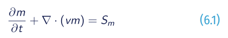
Where m is the sea ice mass per unit area, Sm is a thermodynamic source/sink term and v is velocity. In the case of a single sea ice category the continuity equation for the sea ice distribution takes the basic form:
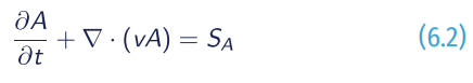
With A is the sea ice concentration and SA is a source/sink term. In addition, the condition A≤1 is imposed. This can be interpreted as a ridging condition since m can increase even if A does not (Hibler, 1979). Together these equations describe the advection of the sea ice in a given velocity field.
The momentum equation is generally written as (Connolley et al., 2004):
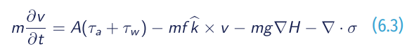
Here k̂ is a unit vector normal to the surface, τa and τw are the air andwater stresses, f is the Coriolis parameter, g is the gravitational acceleration, ∇H is the gradient of the sea surface height and σ is the sea ice stress tensor. The acceleration term on the left-hand side may be set to zero, depending on the model implementation. The last term on the right hand side ∇·σ, describes forces due to internal stress while the other terms are all external factors. Wind and water stresses are generally treated as quadratic drag (e.g., McPhee, 1975). In the absence of internal stress, the sea ice is in “free drift” and the model simplifies drastically. Free drift forecasts have therefore been used for a long time (Grumbine 1998) are still used operationally.
The thermodynamic equation is the heat diffusion equation:
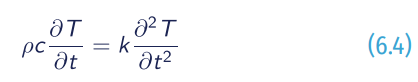
Where ρc is the heat capacity of sea ice or snow and k is the heat conductivity. This equation can be solved in various ways (see Figure 6.3) (e.g., Maykut and Untersteiner, 1971; Semtner, 1976; Bitz and Libscomb, 1999; Winton, 2000; Huwald et al., 2005), discretized in the vertical (Figure 6.3). These take into account different physical properties and numerical solutions in solving the equation.
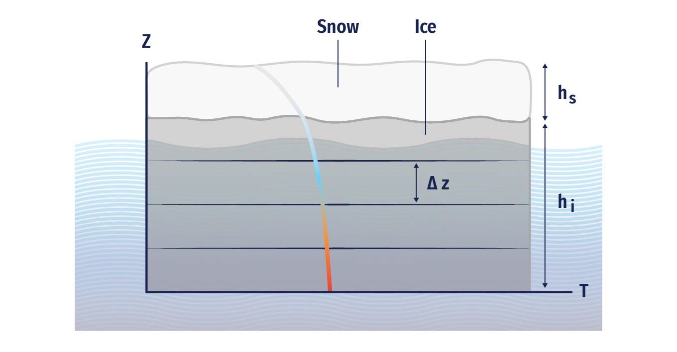
Figure 6.3. Illustration of a vertical temperature profile in a column consisting of sea ice of thickness hi and topped by snow of depth hs. The heat
conduction equation is discretized in the vertical by Δz-thick levels (adapted from Lisæter 2009).
In addition to these grid-scale quantities, many models consider various sub-grid scale information and parameterisations. The most important of those is arguably the ice thickness distribution (ITD). This assumes that each grid cell of the model contains not is of uniform thickness, but of varying thicknesses described by an ice thickness distribution g (see Figure 6.3). This is in principle a continuous distribution of thicknesses, which is modified through dynamic and thermodynamic processes. The governing equation of evolution of the ice thickness distribution is (e.g., Thorndike et al., 1975):
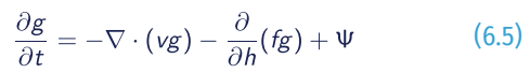
Where f is the thermodynamic growth or melt rate, h is the ice thickness, and 𝚿 is a mechanical redistribution function.
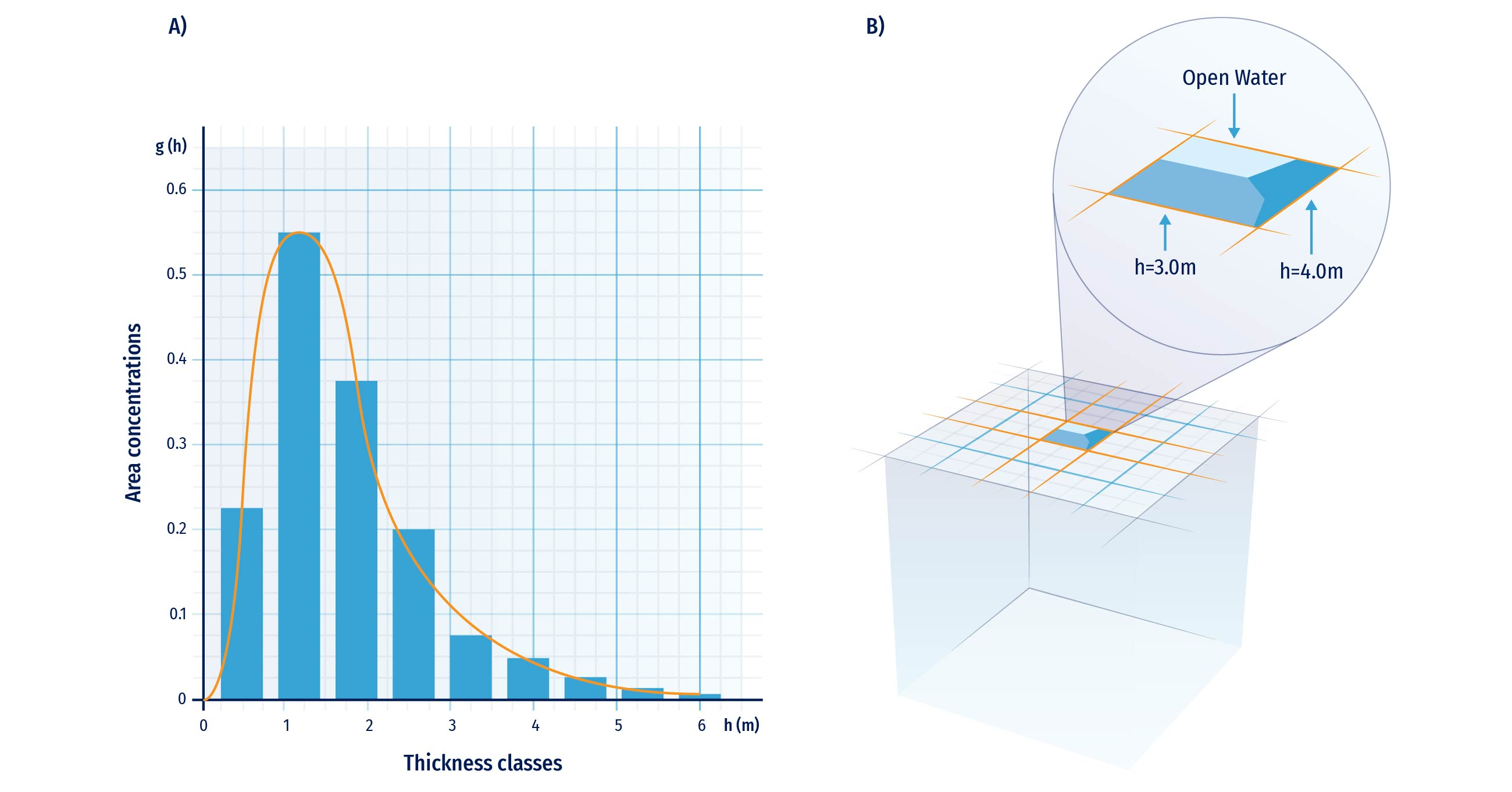
Figure 6.4. Left: a schematic example of an ice thickness distribution, the thickness classes are in x-axis and the y-axis relates to the area concentrations. The continuous distribution is shown with a solid line, while the discretized version is shown in filled bars. Right: illustration of the subgrid-scale ice thickness distribution in a sea ice model (only two classes of 3 and 4 m thickness for the sake of illustration) (adapted from Lisæter, 2009).
In practice, sea ice models must use a discretized version of the ice thickness distribution, resulting in models with several distinct thickness categories (Figure 6.4 right, for a top view of a grid cell). The thickness distribution then becomes (Bitz et al., 2001):
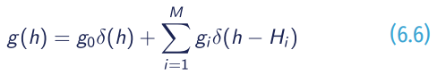
Where M is the number of thickness categories, Mi is the thickness of category i, and δ(h) is the Dirac delta function. Various implementations exist, but the one from Bitz et al., (2001) with five thickness categories remains a popular choice.
In addition to these two basic components, a large number of sub-grid scale processes can and should be represented, depending on the use cases for each model. These include simulation of melt points (Flocco et al., 2010; Hunke et al., 2013), changes in atmospheric and oceanic drag due to sea ice roughness (Tsamados et al., 2014), and salt rejection from freezing sea ice (Vancoppenolle et al. 2009).
6.2.3.2
Sea ice rheology
The relationship between the internal stress and resulting deformation is referred to as rheology. Basically, all continuum, geophysical-scale sea ice models currently employ the VP rheology proposed by Hibler (1979) or some direct descendant of that work. The VP rheology treats the sea ice as a continuum and assumes it deforms in a viscous manner with a high viscosity until the internal stress reaches a plastic threshold, determined by a yield curve which usually has an elliptic shape (see Figure 6.5). Several important improvements have been made to the original VP rheology (e.g. Hunke and Dukowicz, 1997; Lemieux et al., 2010; Bouillon et al., 2013; Kimmritz et al., 2017), but the physical principles remain the same.
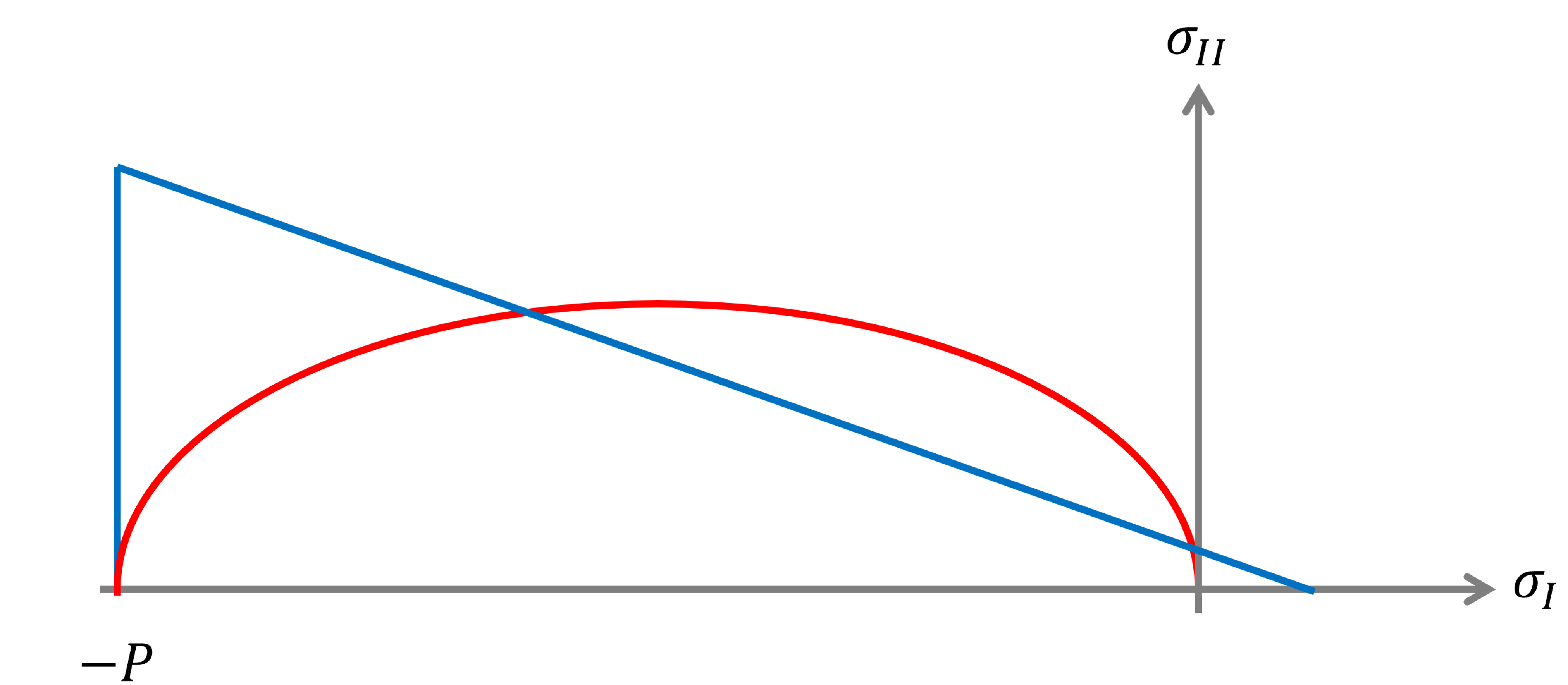
Figure 6.5. Two yield curves commonly associated with sea ice rheology: in red the elliptic yield curve used in the (E)VP models, and in blue a Mohr-Coulomb yield curve, for instance used in the brittle rheology of neXtSIM.
The VP rheology has enjoyed tremendous success and is used for time scales from days to centuries and spatial scales from tens of kilometres to basin scales. However, the VP rheology is not without faults when it comes to both the underlying assumptions (see in particular Coon et al., 2007) and the results it produces. In model inter-comparison studies, there is generally a very large spread - well beyond observed variability - in key prognostic variables such as sea ice thickness, concentration, and drift (Chevallier et al., 2017; Tandon et al., 2018). The sharp gradients in velocities, which are known as LKFs that are related to ridge and lead formation, are also poorly reproduced in any VP-based model running at a coarser resolution than about 2 km - a resolution that is an order of magnitude higher than the observational data (Spreen et al., 2017; Hutter et al., 2019).
Therefore, several authors, such as Tremblay and Mysak (1997), Wilchinsky and Feltham (2004), Schreyer et al. (2006), Girard-Ardhuin and Ezraty (2012), Dansereau et al. (2016), and Ólason et al. (2022), have suggested alternative approaches to the VP rheology. The EAP rheology of Wilchinsky and Feltham (2004) was implemented in the CICE model (Tsamados et al., 2013) and has been used in several studies, although it was not widely adopted yet (Bouchat et al., 2021; Hutter et al. 2021). The brittle rheologies of Girard et al. (2011), Dansereau et al. (2016), and Ólason et al. (2022) have all been implemented in the neXtSIM model (Bouillon and Rampal 2015; Rampal et al., 2019; Ólason et al., 2022) and used for forecasting and scientific research by the team involved in the model. The current neXtSIM version uses the BBM rheology of Ólason et al. (2022).
6.2.3.3
Community sea-ice models
Practically all sea ice models used in modern forecasting platforms are based on the principles described above. They use a Eulerian reference frame and use some version of the VP or the Elastic-Viscous-Plastic (EVP) rheologies. The thermodynamic growth and melt of ice are described through the diffusion of heat between ocean and atmosphere, through the ice. As such, they all follow the same general design philosophy. The main differences exist in the form of different choices of parameterisation and differences in data assimilation approaches.
Today, the CICE model (e.g. Hunke et al., 2021) is likely the most widely used sea ice model for operational forecasts. This model was developed at the Los Alamos National Laboratory and was originally designed to be part of the CCSM. Thanks to its clean and modular design, the model has been used in other multiple modelling systems, as a stand-alone model, part of sea ice-ocean models, and part of climate and earth-system models. The LIM and SI3 models (Rousset et al., 2015), which are part of the NEMO modelling system, are also very widely used, but only within the NEMO modelling system. Other sea-ice models include the SIS (Adcroft et al., 2019), which is part of the GFDL ocean modelling system MOM, the MITgcm sea-ice model (Losch et al., 2010) and the FESOM sea-ice model (FESIM, Danilov et al., 2015).
In contrast, only a few stand-alone sea ice models have used moving Lagrangian coordinates (Hopkins 2004), among which the neXtSIM model (Rampal et al., 2016; Rampal et al., 2019; Ólason et al., 2022) and the DEMSI model (Turner et al., 2022). neXtSIM-F is unique among forecasting models as it uses both a moving Lagrangian mesh and a newly developed brittle rheology, the Brittle Bingham-Maxwell (Williams et al., 2021; Ólason et al., 2022). This setup gives results that are clearly different from the classical systems, and arguably more realistic (Rampal et al., 2016; Rampal et al., 2019; Ólason et al., 2020; Ólason et al., 2022). The key improvement is a much more realistic representation of the deformation statistics of the ice cover, which gives more realistic leads and ridges in the model. Sea ice drift simulated by neXtSIM is also very realistic, and the pan-Arctic ice-thickness distribution is also quite good (Williams et al., 2021).
6.2.3.4
Coupling of sea ice to atmosphere and ocean
Sea ice models are integral parts of Earth system models. The reason for this is that at high latitudes sea ice insulates the relatively warm ocean from the cold atmosphere. Over an unbroken sea ice cover, the atmosphere can therefore cool much more than it could if it was not insulated by the presence of sea ice. This has an impact on all ocean-atmosphere interactions in the polar regions, and therefore a global climate or Earth system model without a sea ice model can simply not function.
Sea ice interacts with the atmosphere through heat, moisture, and momentum exchanges. In summer incoming shortwave radiation melts the ice surface but would warm up the ocean surface in the absence of sea ice. In winter, heat conduction from the ocean and through the ice only results in a very modest amount of heat flux to the atmosphere. However, the dominant heat flux source is radiant cooling through long wave radiation from the surface. This happens because surface cooling through long wave radiation is much more efficient than the heat conduction through ice from the ocean, resulting in a surface that is colder than the lowest layers of the atmosphere. The result is a predominant temperature inversion and a stable atmospheric boundary layer. This reduces even further the latent and sensible heat fluxes from the surface. However, openings in the ice (leads and polynyas) expose the relatively warm ocean surface to the atmospheric boundary layer, which causes mixing and breaks down the stable boundary layer.
Momentum transfer between ice and atmosphere happens through wind stress at the surface of the ice. This is the main driver of ice movement and exerts a drag on the atmosphere, slowing down the wind. The amount of momentum transferred between ice and atmosphere is determined primarily by the stability of the atmospheric boundary layer (Gryanik and Lüpkes, 2017) and the roughness of the ice. While parameterisations and studies on the ice surface roughness have been proposed (Lüpkes et al., 2012, Castellani et al., 2014), consistent and basin-scale observations of the atmospheric drag coefficient over sea ice are currently unavailable (Petty et al., 2017). In a modelling context, our ability to predict ice surface roughness is severely limited, as most ice-atmosphere coupled models do not take surface roughness into account when calculating atmosphere-ice momentum exchanges.
Sea ice interacts with the ocean through heat, fresh-water, and salt exchanges, as well as momentum exchanges. During summer, the mixed layer may warm up due to shortwave heating through openings in the ice. This makes the ice melting from below, causing release of both freshwater and salt into the ocean. In winter, the atmosphere extracts heat from the ocean through the ice, causing new ice to form at the bottom of the existing ice pack. This causes a net heat and freshwater flux out of the ocean. However, most of the salt present in the ocean cannot enter the ice, since the ice is much fresher than the ocean (ca. 15 vs 30 PSS for newly formed ice in the Arctic). This results in a layer of very salty water forming below the ice, which then sinks into the mixed layer. The resulting salt plumes generally reach the bottom of the halocline but may also be mixed into the mixed layer in the presence of turbulence.
Momentum transfer between ice and ocean happens through interface stress between ocean and ice. The momentum coupling of ice and ocean is much stronger than that of ice and atmosphere, and the ice can be considered as the first layer in the ocean’s Ekman spiral. Ice-ocean stress drives most geostrophic flows in ice covered areas, as well as some larger scale circulation patterns.
It is also worth mentioning the interaction between sea ice and ocean waves. Waves entering the ice pack may mechanically fracture it into smaller sea ice floes. This can widen the MIZ, which may also be viewed as the area where the ice is fractured by waves. Fracturing the ice into smaller floes increases the mobility of the ice cover, the momentum transfer between atmosphere, ocean, and ice, and this may cause enhanced melting of the ice through lateral melt. The ice in turn dampens the waves causing an attenuation of the wave amplitude, so that waves will only penetrate a limited distance into the ice pack, depending on the size of the waves and the compactness of the pack. Wave-ice interactions are of major importance in the Southern Ocean, but less so in the Arctic, where much less of the ice edge is exposed to open ocean.
Virtually all climate or earth-system models today include sea-ice models of the classical description above, i.e., a Eulerian reference frame, VP or EVP rheology, and thermodynamics and column physics of varying complexity. They generally include very simplistic formulations for the momentum transfer between atmosphere, ocean, and ice, and no ice-wave interactions. This is true for all the CMIP6 models. In fact, the sea ice models used in today's forecasting models were all designed for climate modelling, the only current exception is the above mentioned neXtSIM model. It is not clear how this lineage of the models affects the quality of their short-term predictions. It could be argued that a good large-scale sea ice model should be able to represent scales from ca. 1 km up to the basin scales and from hours to centuries. This is not the current case, but the discussion of why it is this way and how to address it is still in its infancy (Hunke et al., 2020; Blockley et al., 2020).
6.2.3.5
Model setup
In nearly all forecasting platforms, the sea ice model is coupled to an ocean model. There are platforms that use fully coupled atmosphere-ocean-sea ice models and only a few platforms using a stand-alone sea ice model. The reasons for this are partly historical: most sea ice models are written as parts of ocean models. Ocean forecasting and re-analysis platforms have tended to include a sea ice model from the start, making a dedicated sea ice forecasting platform redundant. In addition, the coupling between sea ice and ocean is quite strong, so running a separate sea ice forecasting platform can bring its own set of challenges. On the other hand, a stand-alone sea ice forecasting platform can be run at a higher resolution and can be used as a technology preview, as in the case of the neXtSIM-F platform.
6.2.4
Ensemble Modelling
Probabilistic forecasts, which are widely used in weather forecasting (Molteni et al., 1996; Leutbecher and Palmer, 2008), are still in their infancy in sea ice forecasting. Probabilistic predictions rely on an ensemble of model simulations (e.g. a Monte Carlo simulation) used to describe the forecast uncertainty stemming from errors in the model parameters, initial and boundary conditions, and any external forcing. The resulting range of model outputs is used to retrieve statistical information, such as the ensemble mean and its spread (i.e. the standard deviation), which are thus used instead of the deterministic forecast to estimate the associated uncertainty (see Figure 6.6). The multiple simultaneous sources of errors usually make the forecast accuracy of the ensemble mean exceed that of the single deterministic prediction (Leith, 1974), although the spread often underestimates the actual forecast error when the sources of error are not all adequately accounted for (Buizza et al., 2005). Monte Carlo techniques are already common practice in different areas (e.g. Dobney et al., 2000; Hackett et al., 2006; Breivik and Allen, 2008; Melsom et al., 2012; Motra et al., 2016; Duraisamy and Iaccarino, 2017) and a common tool for sensitivity analysis.
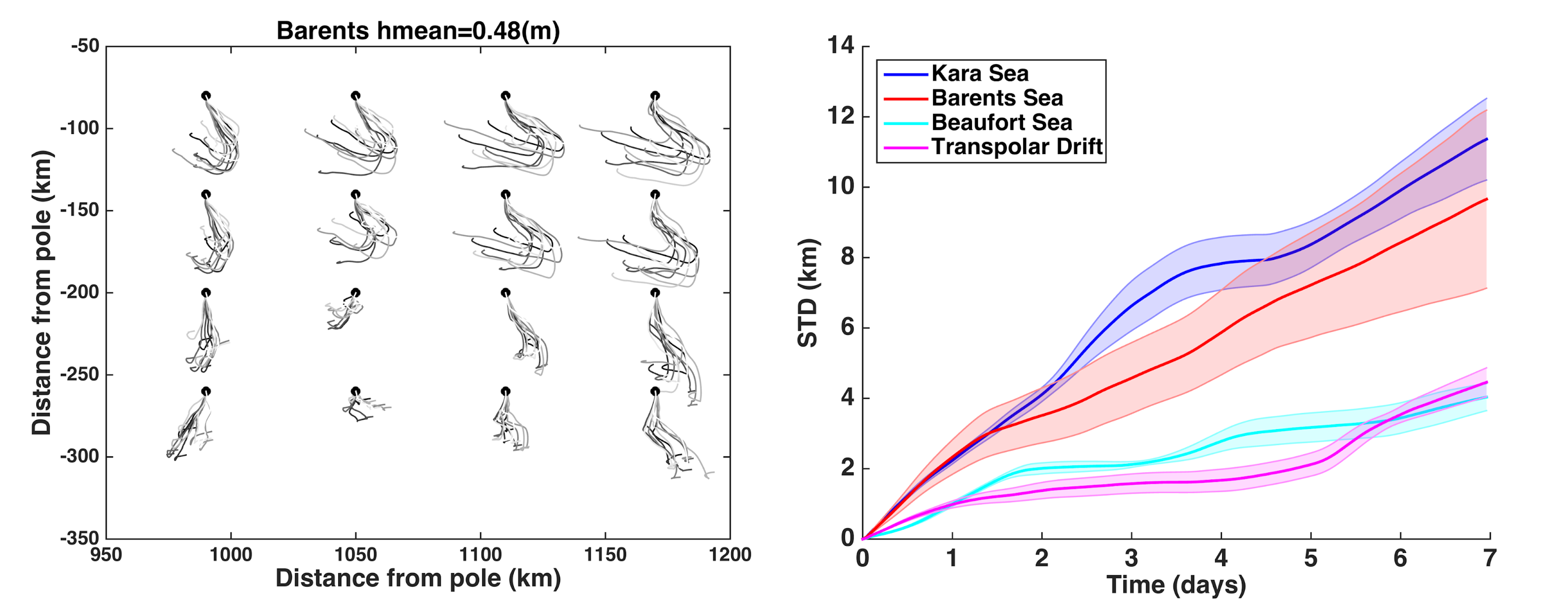
Figure 6.6. Left: example of ice trajectories from an ensemble of 10 members of 7-days sea ice drift of synthetic floats in an area of the Barents Sea from the TOPAZ system using randomly perturbed winds. The mean sea ice thickness is indicated above. Right: illustration of the ensemble spread in end point positions increasing as a function of the forecast length. The uncertainty growth depends strongly on the region (from Bertino et al., 2015).
6.2.5
Data Assimilation systems
As introduced in the previous section, a sea ice forecast needs to regularly assimilate operational observations, which, at present, are mostly satellite data. The most tempting way forward is to insert directly the satellite observed concentrations and thicknesses into the model. However, this is not as easy as it sounds in a complex sea ice code where a large number of model variables are dependent on each other. Hence, various data assimilation methods are used for sea ice models, similar to those used for ocean physical, biogeochemical models or weather models. The most common method is nudging, which is less disruptive than direct insertion: the data are introduced gradually over a given time scale (Lindsay and Zhang, 2006). The nudged model is then assumed to adjust itself progressively using its own equations. But how much can we rely on such adjustments?
When the ocean mixed layer is too warm to sustain sea ice but observations show the presence of sea ice, a data assimilation system updating only sea ice would add sea ice on top of the warm waters, but the huge heat capacity of the ocean would then melt the added sea ice almost immediately. The ocean mixed layer temperature and salinity must be adjusted accordingly. This suggests that when used in a coupled ice-ocean system, assimilation of sea ice observations ought to be coupled in the sense that it should update both the sea ice and the ocean properties consistently. In data assimilation jargon, this means that the sea ice observation should be projected down to the ocean column using a multivariate forecast error covariance matrix.
6.2.5.1
Ensemble-based methods
Dynamical model ensembles are a practical way to estimate the covariances mentioned above. In data assimilation terminology, the state vector must include all prognostic variables of the coupled model (ocean and sea ice variables) and the ensemble of model runs can be used to calculate empirically the cross-covariances between sea ice and ocean variables. Similarly, observations of the ocean are used to update sea ice variables, although this situation is less common. Using an EnKF (see section 5.5.2), Lisæter et al. (2003) demonstrated that the coupled assimilation of sea ice properties can modify the ocean surface temperatures in rather systematic ways (adding sea ice cools down the water), but not ocean salinities. However, according to sea ice halodynamics, the freezing of sea ice injects salty brines to the ocean mixed layer and the melting releases fresher water, but these simple relationships explain only a part of the sea ice-salinity cross-covariances and a relationship may arise in other situations without the intervention of sea ice thermodynamics: the wind may occasionally blow the sea ice on top of more saline water. Sakov et al. (2012) showed how the sea ice-salinity cross-covariance can change sign on either side of the ice edge in the Barents Sea: the sea ice-salinity correlation turns negative on the ocean side because the main process responsible for melting is the advection of warm and saline Atlantic water near the surface, thus the sea ice-salinity correlation is made through the intermediate of the surface temperature variable. The last finding does not hold in locations where the sea ice is isolated from the Atlantic water, but such isolation may not remain forever if the open water mixing reaches these warm waters (Rippeth et al., 2015). The assimilation of sea ice concentrations with the EnKF described in Lisæter et al. (2003) was included in the near-real-time TOPAZ forecasts in 2003.
6.2.5.2
Variational methods
An alternative to ensemble methods is the use of an adjoint model as in the 4D-variational (4D-Var) data assimilation method. The adjoint model and the tangent linear model calculate the sensitivity of observed variables to the control variables within the duration of the assimilation window. If tangent linear and adjoint models are available both for the ocean and the sea ice models, they can exchange information about the interface variables, like the heat, salt, and momentum fluxes. Since these correlations are usually monovariate at the beginning of the assimilation window, the length of the assimilation window should be as long as possible. The most recent experiments report successful applications of the 4D4D-VarVAR in an Arctic regional configuration for durations of one year or longer (Fenty and Heimbach 2013; Fenty et al., 2015); an adjoint model for the EVP sea ice rheology has been introduced later (Toyoda et al. 2019). The advantage of the 4D-Var method is that it returns one optimised model trajectory, which is very useful for oceanographic interpretation (Kauker et al., 2009) and quantitative network design (Kaminski et al., 2015) but, to our knowledge, 4D-Var is not used for operational sea ice-ocean forecasting.
A computationally simplified variant of 4D-Var is known as 3D-Var, in which the same increment is used to compute the model equivalent of the observation-minus-reference state differences at all times in the assimilation. Owing to the relatively low cost of the scheme compared with the full 4D-Var, 3D-Var is commonly used by operational forecasting centres around the world (Usui et al., 2006; Mogensen et al., 2012; Hebert et al., 2015; Tonani et al., 2015; Waters et al., 2015; Smith et al., 2016, see Table 6.3 below).
6.2.5.3
Challenges with coupled data assimilation
Coupled multivariate covariances do not necessarily cure all the troubles of assimilating sea ice observations. Another source of problems is the lack of respect of the traditional Gauss-linear assumptions underlying classical data assimilation methods. By definition, sea ice concentrations have bounded values between zero and one, while other sea ice tracer variables (thickness, snow depth) have positive values only. Ocean temperatures are not allowed below the freezing point. While it should be easy for a monovariate assimilation method, based on a heuristic covariance function, to preserve monotonicity and therefore the bounds of variables (Wackernagel, 2003), an ensemble-based covariance (or a tangent linear model) may generate values out of bounds. Honouring the bounds can be forced by different means, either by nonlinear transformations of the variables (a method called Gaussian anamorphosis in geostatistics; Bertino et al., 2003, Barth et al., 2015) or by including inequality constraints in the cost function (Lauvernet et al., 2009; Simon et al., 2012; Janjic et al., 2014). Altogether, the benefits of multivariate flow-dependent covariances still outbeat the inconvenience of values out of bounds.
There are continuous improvements to data assimilation methods in chaotic high-dimensional systems, such as coupled sea ice-ocean models. But new models and new observations always call for further developments in data assimilation. In particular, sea ice models expressed in Lagrangian grids with automatic remeshing are uncommon targets for data assimilation. Ensemble Kalman Filtering techniques rely on cross-covariances between observed and unobserved variables, which implies that the grid cells have to be uniquely identified across different members of the ensemble. This also becomes difficult when adaptive remeshing is turned on, unless the Lagrangian model output is interpolated on a fixed grid, at the risk of smoothing the very localised kinematic features (long cracks, ridges and leads) that they are meant to simulate (Aydoǧdu et al., 2019). Lagrangian models do not offer any easy differentiation/automatic adjoint capabilities, thus preventing the use of variational techniques. It should also be noted that a coupling framework such as CESM is sufficiently flexible to allow several instances of a model component to be run (for example, the atmosphere) for each instance of another (for example, the ocean), thus allowing to use different data assimilation methods for the sea ice, ocean, land, and atmosphere. An important aspect in view of coupled data assimilation and ensemble forecasting is that the uncertainties are consistent across these compartments; the error statistics at the base of the atmosphere are consistent with those at the surface of the sea ice and similarly between the bottom of the sea ice and the ocean surface. This is possible to enforce if all components of the coupled system use an ensemble to represent the errors.
6.2.6
Validation strategies
Since a measure of RMS errors of sea ice concentrations depend on arbitrary choices made by the person doing the scoring (these errors diminish as more open ocean is included in the validation area), more targeted sea ice validation metrics express the skill as distance of the forecast from the observed ice edge (Dukhovskoy et al., 2015). In the Arctic, the skill of the 24-hour forecast of ice edge location is about 50 km for the TOPAZ (including both seasonal biases and RMS errors, updated at http://cmems.met.no/ARC-MFC/) and 40 km down to 30 km depending on the input data sources in the ACNFS (Hebert et al. 2015; Posey et al., 2015), although both methods may differ and be sensitive to special configurations of the ice edge. The area of discrepancy is accepted as an objective metric with the IIEE introduced by Goessling et al. (2016). The dependence of such metrics on spatial scales can be further included in the evaluation using the FSS (Melsom et al., 2019) and an extension of the IIEE metric proposed by Goessling and Jung (2018) for the evaluation of ensemble forecasts of the ice edge. Examples of IIEE and FSS are shown in Figure 6.7.
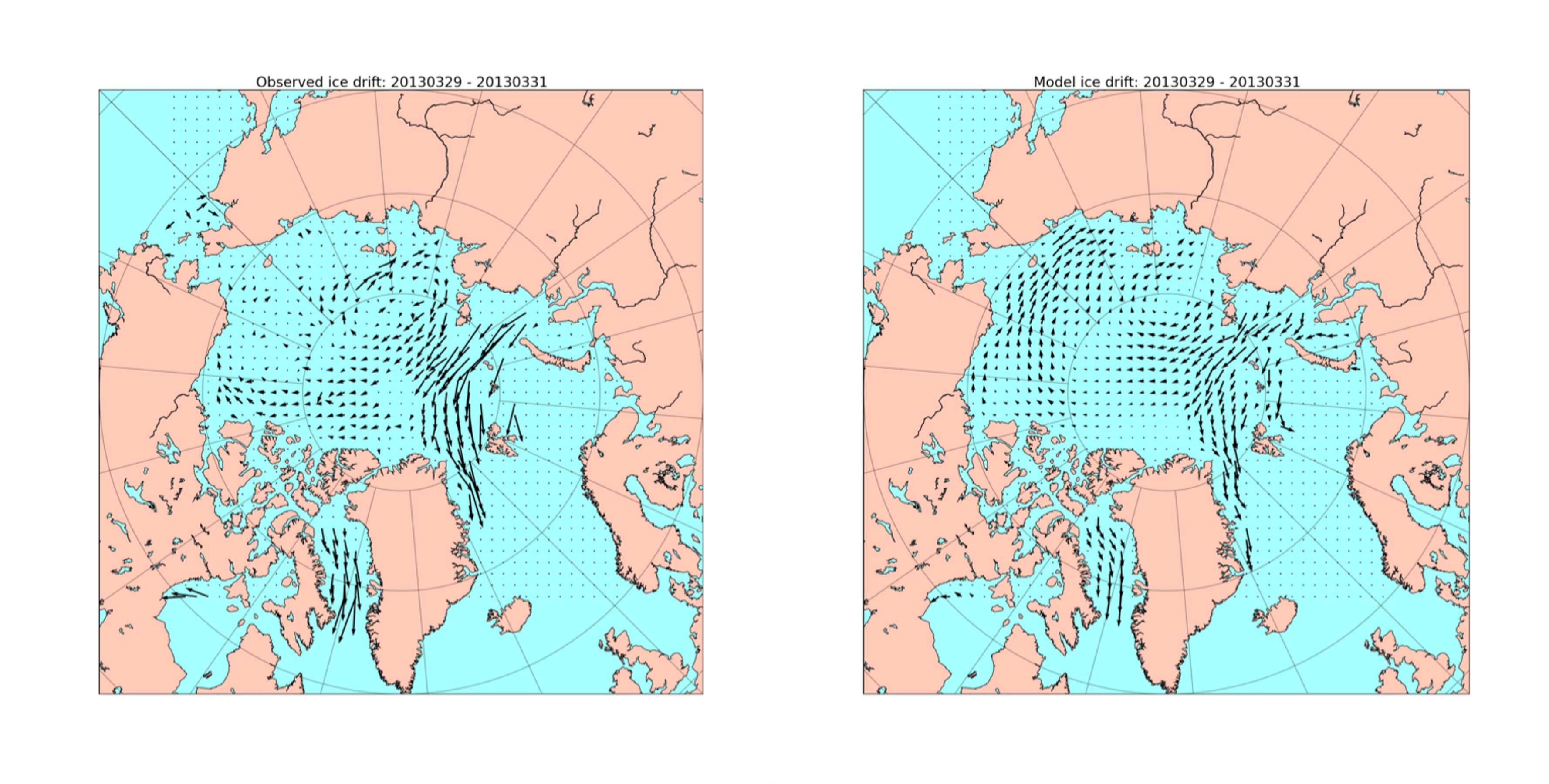
Figure 6.7. Left: example of areas of excess ice (A+) and missing ice (A-) for a given TOPAZ forecast in the European Arctic; the validation data is the Norwegian Ice Charts. Right: associated Fraction Skill Scores showing that the forecast beats persistence at +5 and +9 days lead time irrespective of spatial scales for that specific forecast (both from https://cmems.met.no/ARC-MFC/ - of Copernicus Marine Service).
It should be noted that the metrics related to isolines (like the ice edge, classically defined at the 15% ice concentration isoline, or at other critical values such as 50% and 85%) apply also to other isolines, like the frontier between FYI and MYI, or to theMIZ/pack boundary. Contingency tables are also a valuable approach to the validation of sea ice concentrations (Smith et al., 2016), as well as the threat scores or the Heidke Skill Score.
The forecast skills for sea ice drift have received comparatively less attention but errors in sea ice drift are important, both for their contribution to the displacement of the sea ice edge and for their cumulative contribution to the sea ice thickness distribution. Long climate simulations hint for a seasonal dependence of the forecast skills, also noted in free drift simulations (Grumbine 1998). Biases of sea ice drift have been revealed in IPCC simulations (Tandon et al., 2018) related to the seasonal cycle. To our knowledge, there are no signs that these shortcomings are corrected in recent forecast models (Xie et al., 2017, for the TOPAZ system; Hebert et al., 2015 for the ACNFS), although a review of global reanalysis systems shows that some models simulate correctly the minimum sea ice drift in March (Chevallier et al., 2017). Hebert et al. (2015) also noted that the forecast of drifter positions beats persistence although the forecast of drift speed does not, indicating that the drift direction is better forecasted than the drift speed. How to remedy these shortcomings? Although adjusting the mean speed of sea ice can be easily achieved by tuning the drag coefficients, there is no simple tuning that can make the sea ice accelerate over years or shift its seasonal cycle.
Figure 6.8. Typical Example of a two-day sea ice drift from satellite observations (OSI-SAF, left) and a model (TOPAZ4, right) (courtesy of A. Melsom, MET Norway).
The assimilation of sea ice drift data has been so far less successful than that of sea ice concentrations: Stark et al. (2008) showed a 50% reduction of errors in ice speed but no benefit to ice concentrations and Sakov et al. (2012) indicated a low sensitivity of the sea ice drift to external perturbations in the wind forcing, which points to a shortcoming of the TOPAZ4 version of the EVP sea ice rheology. Qualitatively, the large-scale patterns of sea ice drift can be reproduced by such a model (see a typical situation in Figure 6.8) but the observed gradients between areas of low sea ice drift (North of Greenland) and strong sea ice drift (North of the Barents Sea) are smoothed by the model, which tends to simulate intermediate values of the sea ice drift speed. The forecast of 24-hours ice trajectories and locations exhibits an RMS error of 6.3 km in TOPAZ4 (Melsom et al., 2015), which does not seem to beat a simple free drift predictor (5 km in Grumbine, 1998). It should be noted that the validation is done against different data sources (sea ice drift from satellite SAR images versus IABP buoys) and at different periods (years 2012-2015 versus 80’s and 90’s decades). The SIDFEx (Goessling et al., 2020), carried out in the framework of the Multidisciplinary drifting Observatory for the Study of Arctic Climate (MOSAiC) ice camp, has been the first to collect forecasts from international systems and has shown that a consensus forecast could be successfully used to order detailed satellite images of the ice camp in advance. Beyond the use of RMS errors, several alternative metrics for sea ice drift validation have been reviewed by Grumbine (2013). Validation metrics for an ensemble of trajectories from a probabilistic ice drift forecast have been proposed by Rabatel et al. (2018) and refined in Cheng et al. (2020) based on an analogy with Search and Rescue operations, in which the ensemble of trajectories define a search ellipse; the success of the forecast is the probability of containment of the target inside the ellipse.
The forecast of sea ice thickness also suffers from excessive smoothness: thick sea ice is too thin and thin sea ice is too thick (Johnson et al., 2012) and errors reach easily one to two metres. There is a dynamical contribution to these errors with the too high sea ice drift speed North of Greenland exaggerating the transport of thick sea ice into the Beaufort Gyre. However, thermodynamic contributions cannot be excluded either (in particular from snow and melt ponds). More generally, any error in the model initial conditions, atmospheric and ocean boundary conditions or its inherent parameters will eventually accumulate in sea ice thickness biases, which means that different errors can cancel each other and yield a correct sea ice thickness for the wrong reasons. It is worth stressing the important role of snow on sea ice as an effective insulator, its presence can inhibit both the growth and melt of sea ice and thus reduce its seasonal cycle. Snow predictions in sea ice-ocean models are very dependent on the quality of precipitation from weather analyses and forecasts which are difficult to validate and usually vary from one product to another (Lindsay et al., 2014).
6.2.7
Outputs
Information on formats and types of outputs by all kinds of OOFS can be found in Chapter 4. In this Section, we list the variables related to sea ice forecasts:
- sea ice concentration (SIC)
- sea ice thickness (SIT)
- sea ice drift velocity in x- and y- directions (SIUV)
- snow depth (SNOW)
- sea ice age
- sea ice albedo (SIALB)
- sea ice temperature
Sea ice forecasting systems generally comply with CF standards. The CF metadata conventions are a widely used standard for atmospheric, ocean, and climate data. Standard names are defined in a CF Standard Name Table (see 🔗4 ). Standard variable names from the CMIP nomenclature can be found in Notz et al. (2016).
6.2.8
Examples of operational sea ice forecasting systems
Most present day short-term forecast systems (listed in Table 6.3) assimilate sea ice concentration and are therefore expected to perform well at forecasting the ice edge. These systems include the Canadian RIOPS (Smith et al., 2021), the United States ACNFS/GOFS3.1 (Hebert et al., 2015), the Italian GOFS16 (Iovino et al,. 2016) the Global and the Arctic Marine Forecasting System (TOPAZ, Sakov et al. 2012) by the Copernicus Marine Services. Stand-alone sea ice models, like neXtSIM-F (Williams et al., 2021), are also used for forecasting purposes and, given that their control vector excludes the ocean, they can be initialised more flexibly than coupled ice-ocean systems. Baltic forecasting systems are omitted for brevity. Ocean data assimilated are also omitted from Table 6.3.
Table 6.3. List of present-day short-term global and Arctic forecast systems. Note that the output spatial resolution may differ from the native resolution.
| Area | System | Resolution (km) | Model | Assimilation (method and sea ice data) | Variables | Website |
|---|---|---|---|---|---|---|
| Arctic | ArcIOPS | 18 km | MITgcm | LESTKF SIC, SIT | SIC, SID, SIT | https://www.oceanguide.org.cn/IceIndexHome/ThicknessIce |
| Arctic | NOAA (Bob Grumbine) | N/A | Free drift | N/A | SIUV | https://mag.ncep.noaa.gov/ |
| Global | RTOFS | 3.5 km | HYCOM-CICE5 | 3DVAR SIC | SIC, SIT, SIUV | https://polar.ncep.noaa.gov/global/ |
| Arctic | TOPAZ4 | 12.5 km | HYCOM-CICE3 | EnKF SIC, SIUV, SIT | SIC, SIT, SIUV. SNOW, SIALB | https://marine.copernicus.eu/ |
| Arctic | neXtSIM-F | 7.5 km* | neXtSIM | Nudging SIC | SIC, SIT, SIUV, SNOW | https://marine.copernicus.eu/ |
| Global | MOi | 3.5 km | NEMO-LIM2 | SEEK SIC | SIC, SIT, SIUV | https://marine.copernicus.eu/ |
| Global | GIOPS | 12 km | NEMO-CICE4 | 3DVAR SIC | N/A | https://science.gc.ca/ |
| Arctic | RIOPS | 3.5 km | NEMO-CICE4 | 3DVAR SIC | N/A | https://science.gc.ca/site/science/en/concepts |
| Global | GOFS3.1 | 3.5 km | HYCOM-CICE4 | 3DVAR SIC | SIC, SIT, SIUV | https://www7320.nrlssc.navy.mil/GLBhycomcice1-12/ |
| Global | ECMWF | 12 km | NEMO-LIM2 | 3DVAR SIC | SIC, SIT | https://www.ecmwf.int/en/forecasts/datasets/set-i |
| Arctic | DMI | 10 km | HYCOM-CICE4 | Nudging SIC | N/A | https://ocean.dmi.dk/models/hycom.uk.php |
| Global | Met Office coupled DA | 12 km | NEMO-CICE5 | 3DVAR SIC | SIC, SIT, SIUV | https://marine.copernicus.eu/ |
| Global | Met Office FOAM | 3.5 km | NEMO-CICE5 | 3DVAR SIC | N/A | |
| Arctic** | VENUS | 2.5km | IcePOM | N/A | SIC, SIT | https://ads.nipr.ac.jp/venus.mirai/#/mirai |
* Note that the resolution of a Lagrangian triangular mesh is not comparable to square grids, thus the output resolution is 3 km.
** VENUS is deployed on demand.
References
Adcroft, A., Anderson, W., Balaji, V., Blanton, C., Bushuk, M., Dufour, C. O., et al. (2019). The GFDL global ocean and sea ice model OM4.0: Model description and simulation features. Journal of Advances in Modelling Earth Systems, 11, 3167-3211, https://doi.org/10.1029/2019MS001726
Aydoǧdu, A., Carrassi, A., Guider, C.T., Jones, C. K. R. T., and Rampal, P. (2019). Data assimilation using adaptive, non-conservative, moving mesh models. Nonlinear Processes in Geophysics, 26(3), 175-193, https://doi.org/10.5194/npg-26-175-2019
Barth, A., Canter, M., Van Schaeybroeck, B., Vannitsem, S., Massonnet, F., Zunz, V., Mathiot, P., Alvera-Azcárate, A., Beckers, J.-M. (2015). Assimilation of sea surface temperature, ice concentration and ice drift in a model of the Southern Ocean. Ocean Modelling, 93, 22-39, https://doi.org/10.1016/j.ocemod.2015.07.011
Bertino, L., Bergh, J., and Xie, J. (2015). Evaluation of uncertainties by ensemble simulation, ART JIP Deliverable 3.3. NERSC, Bergen, Norway.
Bertino, L., Evensen, G., Wackernagel, H. (2003). Sequential Data Assimilation Techniques in Oceanography. International Statistical Review 71(2), 223-241, http://www.jstor.org/stable/1403885
Bitz, C. M. and Lipscomb, W. H. (1999). An energy-conserving thermodynamic model of sea ice. Journal of Geophysical Research: Oceans, 104(C7), 15669-15678, https://doi.org/10.1029/1999JC900100
Bitz, C. M., Holland, M. M., Weaver, A. J., and Eby, M. (2001). Simulating the ice-thickness distribution in a coupled climate model. Journal of Geophysical Research: Oceans, 106(C2), 2441-2463, https://doi.org/10.1029/1999JC000113
Blockley, E. W. and Peterson, K. A. (2018). Improving Met Office seasonal predictions of Arctic sea ice using assimilation of CryoSat-2 thickness. The Cryosphere, 12, 3419-3438, https://doi.org/10.5194/tc-12-3419-2018
Blockley, E., Vancoppenolle, M., Hunke, E., Bitz, C., Feltham, D., Lemieux, J., Losch, M., Maisonnave, E., Notz, D., Rampal, P., Tietsche, S., Tremblay, B., Turner, A., Massonnet, F., Ólason, E., Roberts, A., Aksenov, Y., Fichefet, T., Garric, G., Iovino, D., Madec, G., Rousset, C., Salas y Melia, D., Schroeder, D. (2020). The future of sea ice modeling: Where do we go from here? Bulletin of the American Meteorological Society, 101, E1302-E1309, https://doi.org/10.1175/BAMS-D-20-0073.1
Bouchat, A., Hutter, N.C., Chanut, J., Dupont, F., Dukhovskoy, D. S., Garric, G., Lee, Y. J., Lemieux, J.-F., Lique, C., Losch, M., Maslowski, W., Myers, P. G., Ólason, E., Rampal, P., Rasmussen, T.A.S., Talandier, C., Tremblay, B. (2021). Sea Ice Rheology Experiment (SIREx), Part I: Scaling and statistical properties of sea-ice deformation fields. Journal of Geophysical Research: Oceans,127(4), e2021JC017667, https://doi.org/10.1029/2021JC017667
Bouillon, S., Fichefet, T., Legat, V., and Madec, G. (2013). The elastic-viscous-plastic method revisited. Ocean Modelling, 71, 2-12, https://doi.org/10.1016/j.ocemod.2013.05.013
Bouillon, S., and Rampal, P. (2015). On producing sea ice deformation data sets from SAR-derived sea ice motion. The Cryosphere, 9, 663-673, https://doi.org/10.5194/tc-9-663-2015
Breivik, Ø. and Allen, A. A. (2008). An operational search and rescue model for the Norwegian Sea and the North Sea. Journal of Marine Systems, 69(1-2), 99-113, https://doi.org/10.1016/j.jmarsys.2007.02.010
Buizza, R., Houtekamer, P. L., Pellerin, G., Toth, Z., Zhu, Y., and Wei, M. (2005). A Comparison of the ECMWF, MSC, and NCEP Global Ensemble Prediction Systems. Monthly Weather Review, 133(5), 1076-1097, https://doi.org/10.1175/MWR2905.1
Castellani, G., Lüpkes, C., Gerdes, R., Hendricks, S. (2014). Variability of Arctic sea ice topography and its impact on the atmospheric surface drag. Journal of Geophysical Research: Ocean, 119(10), 6743-6762, https://doi.org/10.1002/2013JC009712
Cavalieri, D. J., Parkinson, C. L. (2012). Arctic Sea ice variability and trends, 1979-2010. The Cryosphere, 6,881-889, https://doi.org/10.5194/tc-6-881-2012
Cheng, S., Aydoğdu, A., Rampal, P., Carrassi, A., Bertino, L. (2020). Probabilistic Forecasts of Sea Ice Trajectories in the Arctic: Impact of Uncertainties in Surface Wind and Ice Cohesion. Oceans, 1(4), 326-342, https://doi.org/10.3390/oceans1040022
Chevallier, M., and Salas-Melia, D. (2012). The role of sea ice thickness distribution in the Arctic sea ice potential predictability: A diagnostic approach with a coupled GCM. Journal of Climate, 25(8), 3025-3038, https://doi.org/10.1175/JCLI-D-11-00209.1
Chevallier, M., Smith, G. C., Dupont, F., Lemieux, J.-F., Forget, G., Fujii, Y., et al. (2017). Intercomparison of the Arctic sea ice cover in global ocean-sea ice reanalyses from the ORA-IP project. Climate Dynamics, 49, 1107-1136, https://doi.org/10.1007/s00382-016-2985-y
Connolley, W. M., Gregory, J. M., Hunke, E., McLaren, A. J. (2004). On the Consistent Scaling of Terms in the Sea-Ice Dynamics Equation. Journal of Physical Oceanography, 34(7), 1776-1780, https://doi.org/10.1175/1520-0485(2004)034<1776:OTCSOT>2.0.CO;2
Coon, M. D., Maykut, G. A., Pritchard, R. S., Rothrock, D. A., Thorndike, A. S. (1974). Modeling the pack ice as an elastic-plastic material. AIDJEX Bulletin, 24, 1-106, Univ. of Wash., Seattle, 1974.
Coon, M., Kwok, R., Levy, G., Pruis, M., Schreyer, H., Sulsky, D. (2007). Arctic Ice Dynamics Joint Experiment (AIDJEX) assumptions revisited and found inadequate. Journal of Geophysical Research: Ocean, 112, C11S90, https://doi.org/10.1029/2005JC003393
Danilov, S., Wang, Q., Timmermann, R., Iakovlev, N., Sidorenko, D., Kimmritz, M., Jung, T., and Schröter, J. (2015). Finite-Element Sea Ice Model (FESIM), version 2. Geoscientific Model Development, 8, 1747-1761, https://doi.org/10.5194/gmd-8-1747-2015
Dansereau, V., Weiss, J., Saramito, P., and Lattes, P. (2016). A Maxwell elasto-brittle rheology for sea ice modelling. The Cryosphere, 10, 1339-1359, https://doi.org/10.5194/tc-10-1339-2016
Dobney, A., Klinkenberg, H., Souren, F., and Van Borm, W. (2000). Uncertainty calculations for amount of chemical substance measurements performed by means of isotope dilution mass spectrometry as part of the PERM project. Analytica chimica acta, 420, 89-94.
Dukhovskoy, D. S., Ubnoske, J., Blanchard-Wrigglesworth, E., Hiester, H. R., and Proshutinsky, A. (2015). Skill metrics for evaluation and comparison of sea ice models. Journal of Geophysical Research: Oceans, 120(9), 5910-5931. https://doi.org/10.1002/2015JC010989
Duraisamy, K. A., and Iaccarino, G. (2017). Assessing turbulence sensitivity using stochastic Monte Carlo analysis. Physical Review Fluids, https://arxiv.org/abs/1704.05187
Feltham, D. L., Untersteiner, N., Wettlaufer, J. S., and Worster, M. G. (2006). Sea ice is a mushy layer. Geophysical Research Letters, 33(14), L14501, ISSN 0094-8276, https://doi.org/10.1029/2006GL026290
Fenty, I., and Heimbach, P. (2013). Coupled sea ice–ocean state estimation in the Labrador Sea and Baffin Bay. Journal of Physical Oceanography, 43(5), 884-904, https://doi.org/10.1175/JPO-D-12-065.1
Fenty, I., Menemenlis, D., and Zhang, H. (2015). Global coupled sea ice-ocean state estimation. Climate Dynamics, 49, 931-956, https://doi.org/10.1007/s00382-015-2796-6
Flocco, D., Feltham, D., Turner, A. (2010). Incorporation of a physically based melt pond scheme into the sea ice component of a climate model. Journal of Geophysical Research: Oceans, 115, C08012, https://doi.org/10.1029/2009JC005568
Gautier, D. L., Bird, K. J., Charpentier, R. R., Grantz, A., Houseknecht, D. W., Klett, T. R., … Wandrey, C. J. (2009). Assessment of Undiscovered Oil and Gas in the Arctic. Science, 324, 1175-1179, https://doi.org/10.1126/science.1169467
Girard, L., Bouillon, S., Weiss, J., Amitrano, D., Fichefet, T., and Legat, V. (2011). A new modeling framework for sea-ice mechanics based on elasto-brittle rheology. Annals of Glaciology, 52, 123-132, doi:10.3189/172756411795931499
Girard-Ardhuin, F., and Ezraty, R. (2012). Enhanced Arctic Sea Ice Drift Estimation Merging Radiometer and Scatterometer Data. IEEE Transactions on Geoscience and Remote Sensing, 50(7), 2639-2648, doi:10.1109/TGRS.2012.2184124
Goessling H., Tietsche, S., Day, J.J., Hawkins, E., Jung, T. (2016). Predictability of the Arctic sea ice edge. Geophysical Research Letters, 43(4), 1642-1650, https://doi.org/10.1002/2015GL067232
Goessling, H. F., and Jung, T. (2018). A probabilistic verification score for contours: Methodology and application to Arctic ice-edge forecast. Quarterly Journal of the Royal Meteorological Society, 144, 735-743, https://doi.org/10.1002/qj.3242
Goessling, H. F. and the SIDFEx Team (2020). Making Use and Sense of 75,000 Forecasts of the Sea Ice Drift Forecast Experiment (SIDFEx), EGU General Assembly 2020, Online, 4-8 May 2020, EGU2020-18867, https://doi.org/10.5194/egusphere-egu2020-18867
Griewank, P. J., Notz, D. (2013). Insights into brine dynamics and sea ice desalination from a 1-D model study of gravity drainage. Journal of Geophysical Research: Oceans, 118, 3370-3386, doi:10.1002/jgrc.20247
Grumbine, R. W. (1998). Virtual Floe Ice Drift Forecast Model Intercomparison. Weather and Forecasting, 13, 886-890, https://doi.org/10.1175/1520-0434(1998)013<0886:VFIDFM>2.0.CO;2
Grumbine, R. W. (2013). Long Range Sea Ice Drift Model Verification. Camp. Springs, Maryland.
Guerreiro, K., Fleury, S., Zakharova, E., Rémy, F., and Kouraev, A. (2016). Potential for estimation of snow depth on Arctic sea ice from CryoSat-2 and SARAL/AltiKa missions. Remote Sensing of Environment, 186, 339-349, https://doi.org/10.1016/j.rse.2016.07.013
Gryanik, V. M., and Lüpkes, C. (2017). An Efficient Non-iterative Bulk Parametrization of Surface Fluxes for Stable Atmospheric Conditions Over Polar Sea-Ice. Boundary-Layer Meteorology, 166, 301-325, https://doi.org/10.1007/s10546-017-0302-x
Hackett, B., Breivik, Ø., Wettre, C. (2006). Forecasting the drift of objects and substances in the ocean. In E.P. Chassignet and J. Verron (ed.s) “Ocean Weather Forecasting, An Integrated View of Oceanography”, 507-524, Springer, Dordrecht.
Hebert, D. A., Allard, R. A., Metzger, E. J., Posey, P. G., Preller, R. H., Wallcraft, A. J., Phelps, M. W., and Smedstad, O. M. (2015). Short-term sea ice forecasting: An assessment of ice concentration and ice drift forecasts using the U.S. Navy's Arctic Cap Nowcast/Forecast System. Journal of Geophysical Research: Oceans, 120, 8327- 8345, https://doi.org/10.1002/2015JC011283
Herman, A. (2015). Discrete-Element bonded particle Sea Ice model DESIgn, version 1.3a - model description and implementation. Geoscientific Model Development, 9, 1219–1241, https://doi.org/10.5194/gmd-9-1219-2016
Hibler, W. D. (1979). A dynamic thermodynamic sea ice model. Journal of Physical Oceanography, 9, 817-846.
Hopkins, M. (2004). A discrete element Lagrangian sea ice model. Engineering Computations, 21, 409-421, https://doi.org/10.1108/02644400410519857
Hunke, E., and Dukowicz, J. (1997). An elastic-viscous-plastic model for sea ice dynamics. Journal of Physical Oceanography, 27(9), 1849-1867, https://doi.org/10.1175/1520-0485(1997)027<1849:AEVPMF>2.0.CO;2
Hunke, E., Hebert, D., Lecomte, O. (2013). Level-ice melt ponds in the Los Alamos sea ice model, CICE. Ocean Modelling, 71, 26-42, https://doi.org/10.1016/j.ocemod.2012.11.008
Hunke, E., Allard, R., Blain, P. et al. (2020). Should Sea-Ice Modeling Tools Designed for Climate Research Be Used for Short-Term Forecasting? Current Climate Change Reports, 6, 121-136, https://doi.org/10.1007/s40641-020-00162-y
Hunke, E., Allard, R., Bailey, D.A., Blain, P., Craig, A., Dupont, F., DuVivier, A., Grumbine, R., Hebert, D., Holland, M., Jeffery, N., Lemieux, J.F., Osinski, R., Rasmussen, T., Ribergaard, M., Roberts, A., Denise, W. (2021). CICE Version 6.3.0. http://doi.org/10.5281/zenodo.1205674
Hutter, N., Losch, M., and Menemenlis, D. (2018). Scaling properties of Arctic sea ice deformation in a high-resolution viscous-plastic sea ice model and in satellite observations. Journal of Geophysical Research: Oceans, 123, 672-687, https://doi.org/10.1002/2017JC013119
Hutter, N., Zampieri, L., Losch, M. (2019). Leads and ridges in Arctic sea ice from RGPS data and a new tracking algorithm. The Cryosphere, 13, 627-645, https://doi.org/10.5194/tc-13-627-2019
Huwald, H., Tremblay, L.-B., Blatter, H. (2005). A multilayer sigma-coordinate thermodynamic sea ice model: Validation against Surface Heat Budget of the Arctic Ocean (SHEBA)/Sea Ice Model Intercomparison Project Part 2 (SIMIP2) data. Journal of Geophysical Research: Oceans, 110, C05010, https://doi.org/10.1029/2004JC002328
Iovino, D., Masina, S., Storto, A., Cipollone, A., and Stepanov, V. N. (2016). A 1/16° eddying simulation of the global NEMO sea-ice–ocean system. Geoscientific Model Development, 9, 2665–2684, https://doi.org/10.5194/gmd-9-2665-2016
Ivanova, N., Johannessen, O. M., Pedersen, L. T., and Tonboe, R. T. (2014). Retrieval of Arctic Sea Ice Parameters by Satellite Passive Microwave Sensors: A Comparison of Eleven Sea Ice Concentration Algorithms, IEEE Transactions on Geoscience and Remote Sensing, 52, 7233-7246, doi:10.1109/TGRS.2014.2310136
Ivanova, N., Pedersen, L. T., and Tonboe, R. T. (2015). Inter-comparison and evaluation of sea ice algorithms: towards further identification of challenges and optimal approach using passive microwave observations. The Cryosphere, 9, 1797-1817, https://doi.org/10.5194/tc-9-1797-2015
Janjić, T., McLaughlin, D., Cohn, S. E., and Verlaan, M. (2014). Conservation of Mass and Preservation of Positivity with Ensemble-Type Kalman Filter Algorithms. Monthly Weather Review,142(2), 755-773, https://doi.org/10.1175/MWR-D-13-00056.1
Jenouvrier, S., Holland, M., Strœve, J., Barbraud, C., Weimerskirch, H., Serreze, M., Caswell, H. (2012). Effects of climate change on an emperor penguin population: analysis of coupled demographic and climate models. Available at https://core.ac.uk/download/pdf/9584173.pdf
Johnson, M., Proshutinsky, A., Aksenov, Y., Nguyen, A.T., Lindsay, R., Haas, C., Zhang, J., Diansky, N., Kwok, R., Maslowski, W., Häkkinen, S., Ashik, I., de Cuevas, B. (2012). Evaluation of Arctic sea ice thickness simulated by Arctic Ocean Model Intercomparison Project models. Journal of Geophysical Research: Oceans, 117(C8), https://doi.org/10.1029/2011JC007257
Kaminski, T., Kauker, F., Eicken, H., and Karcher, M. (2015). Exploring the utility of quantitative network design in evaluating Arctic sea ice thickness sampling strategies. The Cryosphere, 9, 1721 1733, https://doi.org/10.5194/tc-9-1721-2015
Kauker, F., Kaminski, T., Karcher, M., Giering, R., Gerdes, R., and Voßbeck, M. (2009). Adjoint analysis of the 2007 all time Arctic sea-ice minimum. Geophysical Research Letters, 36, L03707, doi:10.1029/2008GL036323
Kimmritz, M., Losch, M., Danilov, S. (2017). A comparison of viscous-plastic sea ice solvers with and without replacement pressure. Ocean Modelling, 115, 59-69, https://doi.org/10.1016/j.ocemod.2017.05.006
Kjesbu, O.S., Bogstad, B., Devine, J.A., Gjøsæter, H., Howell, D., Ingvaldsen, R.B., Nash, R.D. M., and Skjæraasen, J. E. (2014). Synergies between climate and management for Atlantic cod fisheries at high latitudes. Proceedings of the National Academy of Sciences of the United States of America,111(9), 3478-3483, https://doi.org/10.1073/pnas.1316342111
Korosov, A. A., and Rampal, P. (2017). A Combination of Feature Tracking and Pattern Matching with Optimal Parametrization for Sea Ice Drift Retrieval from SAR Data. Remote Sensing, 9(258), https://doi.org/10.3390/rs9030258
Kundzewicz, Z. W., Mata, L. J., Arnell, N. W., Doll, P., Kabat, P., Jimenez, B., Miller, K., Oki, T., Zekai, S. and Shiklomanov, I. (2007) Freshwater resources and their management. In: Parry, M. L., Canziani, O. F., Palutikof, J. P., van der Linden, P. J. and Hanson, C. E. (eds.) “Climate Change 2007: Impacts, Adaptation and Vulnerability. Contribution of Working Group II to the Fourth Assessment Report of the Intergovernmental Panel on Climate Change”. Cambridge University Press, 173-210, ISBN 9780521880091
Kurtz, N., Farrell, S. L., Studinger, M., Galin, N., Harbeck, J. P., Lindsay, R., Onana, V. D., Panzer, B., and Sonntag, J. G. (2013). Sea ice thickness, freeboard, and snow depth products from Operation IceBridge airborne data. The Cryosphere, 7, 1035-1056, https://doi.org/10.5194/tc-7-1035-2013
Kwok, R. (2006). Contrasts in sea ice deformation and production in the Arctic seasonal and perennial ice zones. Journal of Geophysical Research: Oceans, 112(C2), https://doi.org/10.1029/2005JC003172
Kwok, R., Cunningham, G. F., Zwally, H. J., and Yi, D. (2007). Ice, Cloud, and land Elevation Satellite (ICESat) over Arctic sea ice: Retrieval of freeboard. Journal of Geophysical Research: Oceans, 112(C12), https://doi.org/10.1029/2006JC003978
Lauvernet, C., Brankart, J.-M. M., Castruccio, F., Broquet, G., Brasseur, P., and Verron, J. (2009). A truncated Gaussian filter for data assimilation with inequality constraints: Application to the hydrostatic stability condition in ocean models. Ocean Modelling, 27(1-2), 1-17. https://doi.org/https://doi.org/10.1016/j.ocemod.2008.10.007
Laxon S. W., Giles, K. A., Ridout, A. L., Wingham, D. J., Willatt, R., Cullen, R., Kwok, R., Schweiger, A., Zhang, J., Haas, C., Hendricks, S., Krishfield, R., Kurtz, N., Farrell S., and Davidson, M. (2013). CryoSat-2 estimates of Arctic sea ice thickness and volume. Geophysical Research Letters, 40, 732-737, https://doi.org/10.1002/grl.50193
Leith, C. E. (1974). Theoretical skill of Monte Carlo forecasts. Monthly Weather Review, 102(6), 409-418, https://doi.org/10.1175/1520-0493(1974)102<0409:TSOMCF>2.0.CO;2
Lemieux, J.-F., Tremblay, B., Sedlácek, J., Tupper, P., Thomas, S., Huard, D., and Auclair, J.-P. (2010). Improving the numerical convergence of viscous-plastic sea ice models with the Jacobianfree Newton Krylov method. Journal of Computational Physics, 229(8), 2840-2852, https://doi.org/10.1016/j.jcp.2009.12.011
Leutbecher, M., and Palmer, T. N. (2008). Ensemble forecasting. Journal of Computational Physics, 227(7), 3515-3539, https://doi.org/10.1016/j.jcp.2007.02.014
Lindsay, R. W., and Zhang, J. (2006). Assimilation of Ice Concentration in an Ice-Ocean Model. Journal of Atmospheric and Oceanic Technology, 23(5), 742-749, https://doi.org/10.1175/JTECH1871.1
Lindsay, R., Wensnahan, M., Schweiger, A., and Zhang, J. (2014). Evaluation of seven different atmospheric reanalysis products in the Arctic. Journal of Climate, 27(7), 2588-2606, https://doi.org/10.1175/JCLI-D-13-00014.1
Lisæter, K. A., Rosanova, J., Evensen, G. (2003). Assimilation of ice concentration in a coupled ice-ocean model, using the Ensemble Kalman filter. Ocean Dynamics, 53, 368-388, https://doi.org/10.1007/s10236-003-0049-4
Lisæter, K. A. (2009). A multi-category sea-ice model. Technical report 304. NERSC, Thormøhlensgt. 47, N-5006 Bergen, Norway.
Losch, M., D. Menemenlis, J.-M. Campin, P. Heimbach, and C. Hill, 2010. On the formulation of sea-ice models. Part 1: Effects of different solver implementations and parameterizations. Ocean Modelling, 33(1-2), 129-144, https://doi.org/10.1016/j.ocemod.2009.12.008
Lüpkes, C., Gryanik, V. M., Hartmann, J., Andreas, E. L. (2012). A parameterization, based on sea ice morphology, of the neutral atmospheric drag coefficients for weather prediction and climate models. Journal of Geophysical Research: Atmospheres, 117(D13), https://doi.org/10.1029/2012JD017630
Marsan, D., Stern, H., Lindsay, R., Weiss, J. (2004). Scale Dependence and Localization of the Deformation of Arctic Sea Ice. Physical Review Letter, 93(17), https://link.aps.org/doi/10.1103/PhysRevLett.93.178501
Maykut, G. A., and Untersteiner, N. (1971). Some results from a time-dependent thermodynamic model of sea ice. Journal of Geophysical Research (1896-1977), 76,1550-1575, https://doi.org/10.1029/JC076i006p01550
McPhee, M. G. (1975). Ice-ocean momentum transfer for the AIDJEX ice model. AIDJEX Bullettin, 29 , 93-111.
Melsom, A., Counillon, F., LaCasce, J. H., Bertino, L. (2012). Forecasting search areas using ensemble ocean circulation modeling. Ocean Dynamics, 62(8), 1245-1257, https://doi.org/10.1007/s10236-012-0561-5
Melsom, A., Palerme, C., Müller, M. (2019). Validation metrics for ice edge position forecasts. Ocean Science, 15(3), 615-630, https://doi.org/10.5194/os-15-615-2019
Mogensen, U. B., Ishwaran. H., Gerds, T. A. (2012). Evaluating Random Forests for Survival Analysis using Prediction Error Curves. Journal of Statistical Software, 50(11), 1-23, doi:10.18637/jss.v050.i11
Molteni, F., Buizza, R., Palmer, T. N., Petroliagis, T. (1996). The ECMWF Ensemble Prediction System: Methodology and validation. Quarterly Journal of the Royal Meteorological Society, 122, 73-119, https://doi.org/10.1002/qj.49712252905
Motra, H. B., Stutz, H., Wuttke, F. (2016). Quality assessment of soil bearing capacity factor models of shallow foundations. Soils and Foundations, 56(2), 265-276, https://doi.org/10.1016/j.sandf.2016.02.009
Mueter, F. J., Litzow, M. A. (2008). Sea ice retreat alters the biogeography of the Bering Sea continental shelf. Ecological Applications, 18(2), 309-20, https://doi.org/10.1890/07-0564.1
Notz, D., and Worster, M. G. (2009). Desalination processes of sea ice revisited. Journal of Geophysical Research: Oceans, 114(C5), https://doi.org/10.1029/2008JC004885
Notz, D., Jahn, A., Holland, M., Hunke, E., Massonnet, F., Stroeve, J., … Vancoppenolle, M. (2016). The CMIP6 Sea-Ice Model Intercomparison Project (SIMIP): Understanding sea ice through climate model simulations. Geoscientific Model Development, 9(9), 3427-3446, https://doi.org/10.5194/gmd-9-3427-2016
Oikkonen, A., Haapala, J., Lensu, M., Karvonen, J., Itkin P. (2017). Small-scale sea ice deformation during N-ICE2015: From compact pack ice to marginal ice zone. Journal of Geophysical Research: Oceans, 122(6), 5105-5120, https://doi.org/10.1002/2016JC012387
Ólason, E., Rampal, P., and Dansereau, V. (2021). On the statistical properties of sea-ice lead fraction and heat fluxes in the Arctic. The Cryosphere, 15, 1053-1064, https://doi.org/10.5194/tc-15-1053-2021
Ólason, E., Boutin, G., Korosov, A., Rampal, P., Williams, T., Kimmritz, M., Dansereau, V. (2022). A new brittle rheology and numerical framework for large-scale sea-ice models. Submitted to Journal of Modelling the Earth System (JAMES), https://doi.org/10.1002/essoar.10507977.2
Overland, J.E, Dethloff, K., Francis, J.A., Hall, R.J., Hanna, E., Kim, S.-J., Screen, J.A., Shepherd, T.G., Vihma, T. (2016). Nonlinear response of mid-latitude weather to the changing Arctic. Nature Climate Change, 6, 992-999, https://doi.org/10.1038/nclimate3121
Perovich, D. K., Richter-Menge, J. A., Jones, K. F., Light, B. (2008). Sunlight, water, and ice: Extreme Arctic sea ice melt during the summer of 2007. Geophysical Research Letters, 35(11), https://doi.org/10.1029/2008GL034007
Petty, A. A., Markus, T., Kurtz, N. (2017). Improving our understanding of Antarctic sea ice with NASA's Operation IceBridge and the upcoming ICESat-2 mission. US CLIVAR Variations, 15(3), doi:10.5065/D6833QQP
Posey, P. G., Metzger, E.J., Wallcraft, A.J., Hebert, D.A., Allard, R.A., Smedstad, O.M., Phelps, M.W., Fetterer, F. , Stewart, J.S., Meier, W.N., and Helfrich, S.R. (2015). Improving Arctic sea ice edge forecasts by assimilating high horizontal resolution sea ice concentration data into the US Navy’s ice forecast systems. The Cryosphere, 9, 1735-1745, https://doi.org/10.5194/tc-9-1735-2015
Rabatel, M., Labbé, S., and Weiss, J. (2015). Dynamics of an Assembly of Rigid Ice Floes. J. Journal of Geophysical Research: Oceans, 120(9), 5887-5909, https://doi.org/10.1002/2015JC010909
Rabatel, M., Rampal, P., Carrassi, A., Bertino, L., and Jones, C.K.R T. (2018). Impact of rheology on probabilistic forecasts of sea ice trajectories: Application for search and rescue operations in the Arctic. The Cryosphere, 12, 935-953, https://doi.org/10.5194/tc-12-935-2018
Rampal, P., Weiss, J., Marsan, D., Lindsay, R., and Stern, H. (2008). Scaling properties of sea ice deformation from buoy dispersion analysis. Journal of Geophysical Research: Oceans, 113(C3), C03002, https://doi.org/10.1029/2007JC004143
Rampal, P., Bouillon, S., Ólason, E., and Morlighem, M. (2016). NeXtSIM: A new Lagrangian sea ice model. The Cryosphere, 10, 1055-1073, https://doi.org/10.5194/tc-10-1055-2016
Rampal, P., Dansereau, V., Olason, E., Bouillon, S., Williams, T., Korosov, A., and Samaké, A. (2019). On the multi-fractal scaling properties of sea ice deformation. The Cryosphere, 13, 2457-2474, https://doi.org/10.5194/tc-13-2457-2019
Richter-Menge, J. A., Perovich, D. K., Elder, B. C., Claffey, K., Rigor, I., Ortmeyer, M. (2006). Ice mass-balance buoys: a tool for measuring and attributing changes in the thickness of the Arctic sea-ice cover. Annals of Glaciology, 44(1), 205-210, doi:10.3189/172756406781811727
Rippeth, T.P. et al. (2015). Tide-mediated warming of Arctic halocline by Atlantic heat fluxes over rough topography. Nature Geoscience, 8(3), 191-194, https://doi.org/10.1038/ngeo2350
Rousset, C., Vancoppenolle, M., Madec, G., Fichefet, T., Flavoni, S., Barthélemy, A., Benshila, R., Chanut, J., Levy, C., Masson, S., and Vivier, F. (2015). The Louvain-La-Neuve sea ice model LIM3.6: global and regional capabilities. Geoscientific Model Development, 8, 2991-3005, https://doi.org/10.5194/gmd-8-2991-2015
Rösel, A., Kaleschke, L., and Birnbaum, G. (2012). Melt ponds on Arctic sea ice determined from MODIS satellite data using an artificial neural network. The Cryosphere, 6, 431-446, https://doi.org/10.5194/tc-6-431-2012
Sakov, P., Counillon, F., Bertino, L., Lisæter, K. A., Oke, P., and Korablev, A. (2012). TOPAZ4: an ocean-sea ice data assimilation system for the North Atlantic and Arctic. Ocean Science, 8, 633-656, https://doi.org/10.5194/os-8-633-2012
Schreyer, H. L., Sulsky, D. L., Munday, L. B., Coon, M. D., Kwok, R. (2006). Elastic-decohesive constitutive model for sea ice. Journal of Geophysical Research: Oceans, 111(C11), https://doi.org/10.1029/2005JC003334
Schulson, E. M., Hibler, W. D. (2017). The fracture of ice on scales large and small: Arctic leads and wing cracks. Journal of Glaciology, 27(127), 319-322, https://doi.org/10.3189/S0022143000005748
Semtner, A. J. (1976). A Model for the Thermodynamic Growth of Sea Ice in Numerical Investigations of Climate. Journal of Physical Oceanography, 6(3), 379-389. https://doi.org/10.1175/1520-0485(1976)006<0379:AMFTTG>2.0.CO;2
Simon, E., Samuelsen, A., Bertino, L., and Dumont, D. (2012). Estimation of positive sum-to-one constrained zooplankton grazing preferences with the DEnKF: a twin experiment. Ocean Science, 8(4), 587-602, https://doi.org/10.5194/os-8-587-2012
Smith, G. C., Roy, F., Reszka, M., Surcel Colan, D., He, Z., Deacu, D., Belanger, J.-M., Skachko, S., Liu, Y., Dupont, F., Lemieux, J.-F., Beaudoin, C., Tranchant, B., Drévillon, M., Garric, G., Testut, C.-E., Lellouche, J.-M., Pellerin, P., Ritchie, H., Lu, Y., Davidson, F., Buehner, M., Caya, A. and Lajoie, M. (2016). Sea ice forecast verification in the Canadian Global Ice Ocean Prediction System. Quarterly Journal of the Royal Meteorological Society, 142(695), 659-671, https://doi.org/10.1002/qj.2555
Smith, G. C., Liu, Y., Benkiran, M., Chikhar, K., Surcel Colan, D., Gauthier, A.-A., Testut, C.-E., Dupont, F., Lei, J., Roy, F., Lemieux, J.-F., and Davidson, F. (2021). The Regional Ice Ocean Prediction System v2: a pan-Canadian ocean analysis system using an online tidal harmonic analysis. Geoscientific Model Development, 14, 1445-1467, https://doi.org/10.5194/gmd-14-1445-2021
Spreen, G., Kwok, R., Menemenlis, D., and Nguyen, A. T. (2017). Sea-ice deformation in a coupled ocean– sea-ice model and in satellite remote sensing data. The Cryosphere, 11, 1553-1573, https://doi.org/10.5194/tc-11-1553-2017
Stark, J. D., Ridley, J., Martin, M., and Hines, A. (2008), Sea ice concentration and motion assimilation in a sea ice-ocean model. Journal of Geophysical Research: Oceans, 113(C5), https://doi.org/10.1029/2007JC004224
Stern, H., Lindsay, R. (2009). Spatial scaling of Arctic sea ice deformation. Journal of Geophysical Research: Oceans, 114(C10), https://doi.org/10.1029/2009JC005380
Sumata, H., Lavergne, T., Girard-Ardhuin, F., Kimura, N., Tschudi, M. A., Kauker, F., Karcher, M., Gerdes, R. (2014). An intercomparison of Arctic ice drift products to deduce uncertainty estimates. Journal of Geophysical Research: Oceans, 119(8), 4887-4921, https://doi.org/10.1002/2013JC009724
Tandon, N. F., Kushner, P. J., Docquier, D., Wettstein, J. J., and Li, C. (2018). Reassessing sea ice drift and its relationship to long-term Arctic sea ice loss in coupled climate models. Journal of Geophysical Research: Oceans, 123, 4338-4359. https://doi.org/10.1029/2017JC013697
Thorndike, A. S., Rothrock, D. A., Maykut, G. A., Colony, R. (1975). The thickness distribution of sea ice. Journal of Geophysical Research: Oceans, 80(33), 4501-4513, https://doi.org/10.1029/JC080i033p04501
Thorndike, A. S., Colony, R. (1982). Sea ice motion in response to geostrophic winds. Journal of Geophysical Research: Oceans, 87(C8), 5845-5852, https://doi.org/10.1029/JC087iC08p05845
Tian-Kunze, X., Kaleschke, L., Maaß, N., Mäkynen, M., Serra, N., Drusch, M., and Krumpen, T. (2014). SMOS-derived thin sea ice thickness: algorithm baseline, product specifications and initial verification. The Cryosphere, 8, 997-1018, https://doi.org/10.5194/tc-8-997-2014
Tonani M., et al. (2015). Status and future of global and regional ocean prediction systems. Journal of Operational Oceanography, 8(sup2), s201-s220, http://doi.org/10.1080/1755876X.2015.1049892
Toyoda, T., Hirose, N., Urakawa, L. S., Tsujino, H., Nakano, H., Usui, N., Fujii, Y., Sakamoto, K., and Yamanaka, G. (2019). Effects of Inclusion of Adjoint Sea Ice Rheology on Backward Sensitivity Evolution Examined Using an Adjoint Ocean-Sea Ice Model. Monthly Weather Review, 147(6), 2145-2162, https://doi.org/10.1175/MWR-D-18-0198.1
Tremblay, L.-B., and Mysak, L. A. (1997). Modeling Sea Ice as a Granular Material, Including the Dilatancy Effect. Journal of Physical Oceanography, 27(11), 2342-2360. https://doi.org/10.1175/1520-0485(1997)027<2342:MSIAAG>2.0.CO;2
Tsamados, M., Feltham, D. L., and Wilchinsky, A. V. (2013). Impact of a new anisotropic rheology on simulations of Arctic sea ice. Journal of Geophysical Research: Oceans, 118, 91-107, https://doi.org/10.1029/2012JC007990
Tsamados, M., Feltham, D. L., Schroeder, D., Flocco, D., Farrell, S. L., Kurtz, N., Bacon, S. (2014). Impact of Variable Atmospheric and Oceanic Form Drag on Simulations of Arctic Sea Ice. Journal of Physical Oceanography, 44, 1329-1353, https://doi.org/10.1175/JPO-D-13-0215.1
Turner, A. K., and Hunke, E. C. (2015). Impacts of a mushy-layer thermodynamic approach in global seaice simulations using the CICE sea-ice model. Journal of Geophysical Research: Oceans, 120, 1253-1275, https://doi.org/10.1002/2014JC010358
Turner, A. K., Hunke, E. C., and Bitz, C. M. (2013). Two modes of sea-ice gravity drainage: A parameterization for large-scale modeling. Journal of Geophysical Research: Oceans, 118, 2279-2294, https://doi.org/10.1002/jgrc.20171
Turner, A. K., Peterson, K. J., and Bolintineanu, D. (2022). Geometric remapping of particle distributions in the Discrete Element Model for Sea Ice (DEMSI v0.0). Geoscientific Model Development, 15, 1953-1970, https://doi.org/10.5194/gmd-15-1953-2022
Urrego-Blanco, J. R., Urban, N. M., Hunke, E. C., Turner, A. K., and Jeffery, N. (2016). Uncertainty quantification and global sensitivity analysis of the Los Alamos sea ice model. Journal of Geophysical Research: Oceans, 121, 2709-2732, https://doi.org/10.1002/2015JC011558
Usui, N., Ishizaki, S., Fujii, Y., Tsujino, H., Yasuda, T., Kamachi, M. (2006). Meteorological Research Institute multivariate ocean variational estimate (MOVE) system: Some early results. Advances in Space Research, 37/4), 806-822, https://doi.org/10.1016/j.asr.2005.09.022
Vancoppenolle, M., Bitz, C. M., and Fichefet, T. (2007). Summer landfast sea ice desalination at Point Barrow, Alaska: Modeling and observations. Journal of Geophysical Research: Oceans, 112(C4), https://doi.org/10.1029/2006JC003493
Vancoppenolle, M., Fichefet, T., Goosse, H., Bouillon, S., Madec, G., and Maqueda, M. A. M. (2009). Simulating the mass balance and salinity of Arctic and Antarctic sea ice. 1. Model description and validation. Ocean Modelling, 27(1-2), 33-53, https://doi.org/10.1016/j.ocemod.2008.10.005
Wackernagel, H. (2003). Multivariate Geostatistics. An Introduction with Applications. Springer Science & Business Media, 12 feb 2003 - 388 pp.
Waters, J., Lea, D.J., Martin, M.J., Mirouze, I., Weaver, A., and While, J. (2015). Implementing a variational data assimilation system in an operational 1/4 degree global ocean model. Quarterly Journal of the Royal Meteorological Society, 141(687), 333-349, https://doi.org/10.1002/qj.2388
Weiss, J., and Marsan, D. (2004). Scale properties of sea ice deformation and fracturing. Comptes Rendus Physique, 5(7), 735-751, https://doi.org/10.1016/j.crhy.2004.09.005
Wilchinsky, A. V., and Feltham, D. L. (2004). A continuum anisotropic model of sea-ice dynamics. Proceedings of the Royal Society A, 460(2047), https://doi.org/10.1098/rspa.2004.1282
Williams, T., Korosov, A., Rampal, P., Ólason, E. (2021). Presentation and evaluation of the Arctic sea ice forecasting system neXtSIM-F. The Cryosphere, 15, 3207-3227, https://doi.org/10.5194/tc-15-3207-2021
Winton A. (2000). A Reformulated Three-Layer Sea Ice Model. Journal of Atmospheric and Oceanic Technology, 17(4), 525-531, https://doi.org/10.1175/1520-0426(2000)017%3C0525:ARTLSI%3E2.0.CO;2
WMO (1970). Sea-ice nomenclature, terminology, codes and illustrated glossary. WMO Rep. WMO/OMM/ BMO 259, 121 pp.
Xie, J., Bertino, L., Counillon, F., Lisæter, K. A., and Sakov, P. (2017). Quality assessment of the TOPAZ4 reanalysis in the Arctic over the period 1991–2013. Ocean Science, 13(1), 123-144, http://doi.org/10.5194/os-13-123-2017
Zygmuntowska, M., Rampal, P, Ivanova, N., and Smedsrud, L. H. (2014). Uncertainties in Arctic sea ice thickness and volume: new estimates and implications for trends. The Cryosphere, 8, 705-720, https://doi.org/10.5194/tc-8-705-2014
Chapter 6
To start contributing, sharing knowledge and editing the WIKI, please login !
Follow us