
An introduction to the data assimilation concept can be found in Section 4.3. This Section focuses on the numerical characteristics of the DAS largely used in circulation modelling.
CHAPTER
COORDINATORS
COORDINATORS
Stefania Ciliberti
5.5
Data assimilation systems

5.5.1
Basic concepts
In ocean forecasting the objective is to produce an estimate xa of the true state xt of the ocean at initial time to initialise forecasts. Ide et al., 1997, De Mey-Frémaux et al. (1998), and Bouttier and Courtier (2002) provide an extensive introduction to DAS basic concepts and herein are recalled and summarised.
DA consists in calculating the «best» estimate of the state of a physical system, of its evolution in time, given observations and a prognostic numerical model.
The basic objective information that can be used to produce the analysis is a collection of observed values provided by observations of the true state. If the model state is overdetermined by the observations, then the analysis is reduced to an interpolation problem. In most cases the analysis problem is under-determined because data are sparse and only indirectly related to the model variables. In order to make it a well-posed problem, it is necessary to rely on some background information in the form of an a priori estimate of the model state.
A discrete model for the evolution of the ocean from ti to ti+1 is governed by the following Eq. 5.13:
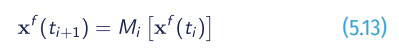
Where x is the so-called state vector (velocities, temperature, salinity, etc., at model grid positions) and M is the corresponding dynamics operator. The state vector has dimension n. The dynamic operator in Eq. 5.13 is commonly non linear and deterministic, while the true ocean state may differ from Eq. 5.13 by random and systematic error.
Observations yo t at time ti are defined by Eq. 5.14:
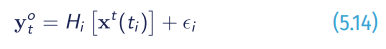
where H is an observation operator and ϵ is a noise process. The observation vector has dimension pi . A major problem of data assimilation is that typically pi<<n. The observation operator H can be also non-linear like M and both can contain explicit time dependence in addition to the implicit dependence via the state vector xf i ≡ xf (ti). The noise process ϵ is commonly used to have zero mean and we denote its covariance matrix by R: it consists of instrumental and representativeness errors which covariance matrices are E and F, respectively, with R=E+F.
The key of the analysis is the use of discrepancies between observations and state vector:

When calculated with the background xb it is called innovations and with the analysis xa analysis residuals.
In the following, we present two data assimilation types of approaches: the sequential methods and the variational methods.
5.5.2
Sequential methods
Several schemes have been proven useful and implemented using a sequential-estimation approach including the Bluelink Ocean Data Assimilation System (BODAS) (Oke et al., 2008) and the Singular Evolutive Extended Kalman (SEEK) filter (Pham et al., 1998). An extensive literature is available on related methods, such as OI (Daley, 1991), EnOI, and EnKF (Evensen, 2003). Following Ide et al., (1997), the true ocean fluid xf is assumed to differ from that of the numerical model (Eq. 13) by stochastic perturbations:
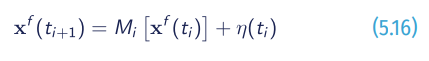
Where η is a noise process with zero mean and covariance matrix Q. The EKF consists of a forecast step based on previously obtained state variables, which include previous assimilation steps, xf (ti+1) and an updated probability function described by Pf (ti):
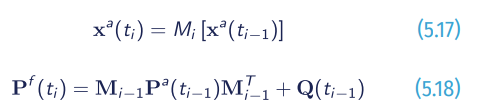
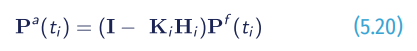
The core of the Kalman Filter method is an update step in which the observations available at time i is blended with the previous information, taking account of their joint probability distributions and carried forward by the forecast step:
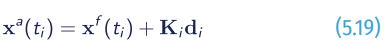
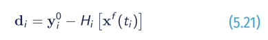
Where the observation residual or innovation vector is defined by:
The Kalman gain Ki is defined by:
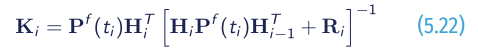
The innovation vector di is evidently a displacement of the modelled forecast toward the observed data, scaled by the Kalman gain. The Kalman gain accounts for the weighting required by the joint probability function for the model and observation variability. In practice, various simplifications are introduced to describe P to overcome the computational burden involved in the matrix calculation (Oke et al., 2008; Pham et al., 1998).
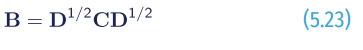
Another example is the OI that is quite frequently used in oceanography and meteorology. It is a particular suboptimal filter, in which the EKF’s error covariance matrix Pf is replaced by an approximation, B, computed as a product of variances placed in the diagonal matrix D and of correlations placed in a matrix C with unit diagonal (Ghil and Malanotte-Rizzoli, 1991):
The state vector is still given by Eq. 5.13. The OI gain writes:
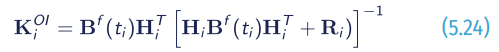
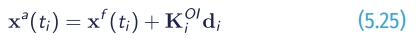
Where HiBf (ti)HT i is evaluated from the correlation model, and the state update is given by:
5.5.3
Variational methods
Several schemes have been implemented using variational methods such as 3D-Var, e.g. the Navy Coupled Ocean Data Assimilation (NCODA) (Cummings, 2005) and the Forecasting Ocean Assimilation Model (FOAM) (Martin et al., 2007). 4D-Var methods are used extensively in Numerical Weather Prediction and are one of the future directions for ocean prediction systems. The NEMOVAR system (Mogensen et al., 2012) is able to handle both categories of variational approaches for the NEMO modelling system.
Following Ide et al. (1997), 4D-Var minimises the objective function J that measures the weighted sum of distance Jb to the background state xb and Jo to the observation yo distributed over a time interval [t0 , tn ]:
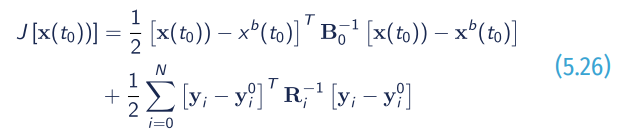
Where yi ≡Hi[x(ti)]. Here B-1 is an a priori weight matrix, with B-1 meant to approximate the error covariance matrix xb, and a minimization is done with respect to the initial state x(to).
Equation 5.25 reflects the imposition of a strong constraint (Sasaki, 1970). Alternative formulations based on a weak constraint are given by Bennett (1992) and by Menard and Daley (1996). Efficient methods for performing the minimization of J require its partial derivatives with respect to the elements of x(to) given by:
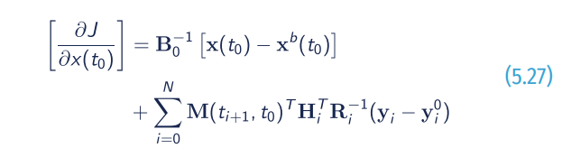
Where:
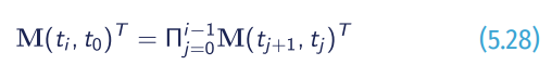
This follows from:
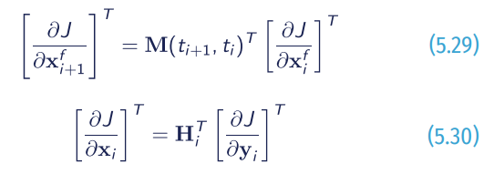
M(ti+1,ti)T is usually called adjoint model and HT i is the adjoint observation operator. 4D-Var reduces to three-dimensional variational assimilation (3D-Var) if the time dimension is taken out.
Figure 5.9 shows an example of 4D-Var capacity: xa is used as the initial state for a forecast, then by construction of 4D-Var one is sure that the forecast will be completely consistent with the model equations and the 4D distribution of observations until the end of the 4D-Var time interval n (the cutoff time).

Figure 5.9. Example of 4D-Var intermittent assimilation in a numerical forecasting system (adapted from Bouttier and Courtier 2002).
5.5.4
Modelling errors
As reported in Bouttier and Courtier (2002), to represent the fact that there is some uncertainty in the background and in the analysis, we need to assume some model of the errors between these vectors.
Given a background field xb just before doing an analysis, we define the vector of errors that separates it from the true state:
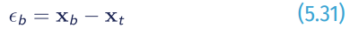
If we are able to repeat each analysis experiment a large number of times, under exactly same conditions but with different realisation of errors generated by unknown causes, b would be different every time. It can be represented through a probability density function (PDF), able to provide all statistics, including the average (or expectation) -b and the variances. A popular model of scalar pdf is the Gaussian function, that can be generalised to a multivariate PDF.
The errors in the background and in the observations are modelled as follows:
- Background errors. They are the estimation errors of the background state, given by the difference between the background state vector and its true value;
- Observation errors. They contain errors in the observation process (i.e instrumental errors), errors in the design of the operator H, and representativeness errors (i.e. discretization errors which prevent x t from being a perfect image of the true state;
- Analysis error. Defined through the trace of the covariance matrix A:
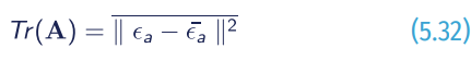
They are the estimation errors of the analysis state, which is what we want to minimize. In a scalar system, the background error covariance is the variance:

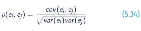
In a multidimensional system, B is a square symmetric matrix with n×n dimension. The diagonal of B contains the variances, while the off-diagonal contains the cross-covariances between a pair of variables in the model. The off-diagonal terms can be transformed into error correlations:
The error statistics are functions of the physical processes governing the meteorological or the ocean state and the observing network. They depend on a priori knowledge of the errors: variances reflect our uncertainty in features of the background or the observations. To estimate statistics, it is necessary to assume that they are stationary over a period and uniform over a domain, so that one can take a number of error realisations and make empirical statistics.
In setting a DAS, the estimated statistics is very difficult and we can rely on diagnostics of an existing data assimilation system using the observational method.
5.5.5
Overview of current data assimilation systems in operational forecasting
Data assimilation techniques, schematically introduced in previous paragraphs and that are widely documented in Daley (1991), Evensen (2003) and Zaron (2011), represent the baseline of the modelling framework with general circulation models for operational forecasting and reanalysis. At international level, the GODAE’s OceanView (Bell et al., 2015) and OceanPredict initiatives have promoted strong synergies with GOOS, ETOOFS and GEO BluePlanet contributing to a value chain from observations, data, information systems, predictions, and scientific assessments to end users, with the aim to promote the use and impact of observations and ocean predictions for societal benefit, and increasing visibility of operational oceanography advances.
Martin et al. (2015) presents an overviewofthe main characteristics of the data assimilation used in each GODAE OceanView systems; this is a list of the adopted numerical techniques:
- Bluelink (Oke et al., 2013) adopts MOM4 ocean model and EnOI algorithm;
- GIOPS (Smith et al., 2016) uses NEMO ocean model and SEEK (with fixed basis) for the ocean component, and 3DVar for assimilation in the ice component;
- ECMWF (Balmaseda et al., 2013) uses NEMO ocean model and 3DVar for the assimilation component (+ bias correction technique);
- FOAM (Waters et al., 2014) uses NEMO ocean model and 3DVar for the assimilation component (+ bias correction technique);
- GOFS (Cummings and Smedstad, 2013) uses HYCOM ocean model with 3DVar data assimilation scheme;
- Mercator Ocean (Lellouche et al., 2013) uses NEMO ocean model with SEEK-FGAT (with fixed basis) and 3DVar bias correction;
- MOVE (Usui et al., 2006) uses MRI COM model and 3DVar data assimilation scheme;
- TOPAZ (Sakov et al., 2012) uses HYCOM with EnKF techniques.
Description of the operational initiatives is also provided at GODAE OceanView website (🔗2 ) and OceanPredict website (🔗3 ).
References
Balmaseda, M. A., Mogensen, K., and Weaver, A.T. (2013). Evaluation of the ECMWF ocean reanalysis system ORAS4. Quarterly Journal of the Royal Meteorological Society, 139, 1132-1161, https://doi.org/10.1002/qj.2063
Balmaseda, M.A., Hernandez, F., Storto , A., Palmer, M.D., Alves, O., Shi, L., Smith, G.C. Toyoda, T., Valdivieso, M., Barnier, B., Behringer, D., Boyer, T., Chang, Y-S., Chepurin, G.A., Ferry, N., Forget, G., Fujii, Y., Good, S., Guinehut, S., Haines, K., Ishikawa, Y., Keeley, S., Köhl, A., Lee, T., Martin, M.J, Masina, S., Masuda, S., Meyssignac, B., Mogensen, K., Parent, L., Peterson, K.A., Tang, Y.M., Yin, Y., Vernieres, G., Wang, X., Waters, J., Wedd, R., Wang, O., Xue, Y., Chevallier, M., Lemieux, J.F., Dupont, F., Kuragano, T., Kamachi, M., Awaji, T., Caltabiano, A., Wilmer-Becker, K., Gaillard, F. (2015). The Ocean Reanalyses Intercomparison Project (ORA-IP). Journal of Operational Oceanography, 8(sup1), s80-s97, https://doi.org/10.1080/1755876X.2015.1022329
Barth, A., Alvera-Azcárate, A., Beckers, J.M., Weisberg, R. H., Vandenbulcke, L., Lenartz, F., and Rixen, M. (2009). Dynamically constrained ensemble perturbations–application to tides on the West Florida Shelf. Ocean Science, 5, 259-270, https://doi.org/10.5194/os-5-259-2009
Bell, M., Schiller, A., Le Traon, P-Y., Smith, N.R., Dombrowsky, E., Wilmer-Becker, K. (2015). An introduction to GODAE OceanView. Journal of Operational Oceanography, 8, 2-11, https://doi.org/10.1080/1755876X.2015.1022041
Bennett, A.F. (1992). Inverse Methods in Physical Oceanography, Cambridge University Press, Cambridge, UK.
Berner, J., G. Shutts, M. Leutbecher, and T. Palmer. (2009). A spectral stochastic kinetic energy backscatter scheme and its impact on flow-dependent predictability in the ECMWF ensemble prediction system. Journal of the Atmospheric Sciences, 66, 603-626, https://doi.org/10.1175/2008JAS2677.1
Bessières, L., Leroux, S., Brankart, J.M., Molines, J.M., Moine, M.P., Bouttier, P.A., Penduff, T., Terray, L., Barnier, B., Sérazin, G. (2017). Development of a probabilistic ocean modelling system based on NEMO 3.5: Application at eddying resolution. Geoscientific Model Development, 10, 1091-1106, https://doi.org/10.5194/gmd-10-1091-2017
Bjerknes, V. (1914). Meteorology as an exact science. Monthly Weather Review, 42(1), 11-14, https://doi.org/10.1175/1520-0493(1914)42<11:MAAES>2.0.CO;2
Blayo, E., and Debreu, L. (1999). Adaptive mesh refinement for finite-difference ocean models: first experiments. Journal of Physical Oceanography, 29(6), 1239-1250, https://doi.org/10.1175/1520-0485(1999)029%3C1239:AMRFFD%3E2.0.CO;2
Blayo, E., and Debreu, L. (2005). Revisiting open boundary conditions from the point of view of characteristic variables. Ocean Modelling, 9(3), 231-252, https://doi.org/10.1016/j.ocemod.2004.07.001
Bouttier, F., and Courtier, P. (2002). Data assimilation concepts and methods, March 1999. ECMWF Education material, 59 pp., https://www.ecmwf.int/en/elibrary/16928-data-assimilation-concepts-and-methods 5.10.
Brankart, J.-M., (2013). Impact of uncertainties in the horizontal density gradient upon low resolution global ocean modelling. Ocean Modelling, 66, 64-76, http://dx.doi.org/10.1016/j.ocemod.2013.02.004
Brankart, J.-M., Candille, G., Garnier, F., Calone, C., Melet, A., Bouttier, P.-A., Brasseur, P., Verron, J., (2015). A generic approach to explicit simulation of uncertainty in the NEMO ocean model. Geoscientific Model Development, 8, 1285-1297, https://doi.org/10.5194/gmd-8-1285-2015
Brassington, G.B., Warren, G., Smith, N., Schiller, A., Oke, P.R. (2005). BLUElink> Progress on operational ocean prediction for Australia. Bulletin of the Australian Meteorological and Oceanographic Society, Vol.18 p. 104.
Buizza, R., Miller, M., Palmer, T.N. (1999). Stochastic representation of model uncertainties in the ECMWF ensemble prediction system. Quarterly Journal of the Royal Meteorological Society, 125, 2887-2908, http://dx.doi.org/10.1002/qj.49712556006
Candille, G., and Talagrand, O. (2005). Evaluation of probabilistic prediction systems for a scalar variable. Quarterly Journal of the Royal Meteorological Society, 131, 2131-2150, https://doi.org/10.1256/qj.04.71
Charria, G., Lamouroux, J., De Mey, P. (2016). Optimizing observational networks combining gliders, moored buoys and FerryBox in the Bay of Biscay and English Channel. J. Mar. Syst., 162, 112-125. http://dx.doi.org/10.1016/j.jmarsys.2016.04.003
Chassignet, E. P., Hurlburt, H. E., Smedstad, O. M., Halliwell, G. R., Hogan, P. J., Wallcraft, A. J., and Bleck, R. (2006). Ocean prediction with the hybrid coordinate ocean model (HYCOM). In “Ocean weather forecasting”, 413-426, Springer, Dordrecht, doi:10.1007/1-4020-4028-8_16
Chelton, D. B., DeSzoeke, R. A., Schlax, M. G., El Naggar, K., and Siwertz, N. (1998). Geographical variability of the first baroclinic Rossby radius of deformation. Journal of Physical Oceanography, 28(3), 433-460, https://doi.org/10.1175/1520-0485(1998)028<0433:GVOTFB>2.0.CO;2
Cheng, S., Aydoğdu, A., Rampal, P., Carrassi, A., Bertino, L. (2020). Probabilistic Forecasts of Sea Ice Trajectories in the Arctic: Impact of Uncertainties in Surface Wind and Ice Cohesion. Oceans, 1, 326- 342, https://doi.org/10.3390/oceans1040022
Ciavatta, S., Torres, R., Martinez-Vicente, V., Smyth, T., Dall'Olmo, G., Polimene, L., and Allen, J. I. (2014). Assimilation of remotely-sensed optical properties to improve marine biogeochemistry modelling. Progresses in Oceanography, 127, 74-95, https://doi.org/10.1016/j.pocean.2014.06.002
Crosnier, L., and Le Provost, C. (2007). Inter-comparing five forecast operational systems in the North Atlantic and Mediterranean basins: The MERSEA-strand1 Methodology. Journal of Marine Systems, 65(1-4), 354-375, https://doi.org/10.1016/j.jmarsys.2005.01.003
Cummings, J. A. (2005). Operational multivariate ocean data assimilation. Quarterly Journal of the Royal Meteorological Society, 131(613), 3583-3604, https://doi.org/10.1256/qj.05.105
Cummings, J.A., and Smedstad, O.M. (2013). Variational data analysis for the global ocean. In: S.K. Park and L. Xu (Eds.), Data Assimilation for Atmospheric, Oceanic and Hydrologic Applications Vol. II., doi:10.1007/978-3-642-35088-7_13, Springer-Verlag Berlin Heidelberg.
Daley, R. (1991). Atmospheric Data Analysis. Cambridge University Press. 457 pp.
Danilov, S., Kivman, G., and Schröter, J. (2004). A finite-element ocean model: principles and evaluation. Ocean Modelling, 6(2), 125-150, https://doi.org/10.1016/S1463-5003(02)00063-X
Debreu, L., Marchesiello, P., Penven, P., and Cambon, G. (2012). Two-way nesting in split-explicit ocean models: Algorithms, implementation and validation. Ocean Modelling, 49, 1-21, https://doi.org/10.1016/j.ocemod.2012.03.003
Debreu, L., Vouland, C., and Blayo, E. (2008). AGRIF: Adaptive grid refinement in Fortran. Computers & Geosciences, 34(1), 8-13, https://doi.org/10.1016/j.cageo.2007.01.009
De Mey-Frémaux and the Groupe MERCATOR Assimilation (1998). Scientific Feasibility of Data Assimilation in the MERCATOR Project. Technical Report, doi: https://doi.org/10.5281/zenodo.3677206
De Mey P., Craig P., Kindle J., Ishikawa Y., Proctor R., Thompson K., Zhu J., and contributors (2007). Towards the assessment and demonstration of the value of GODAE results for coastal and shelf seas and forecasting systems, 2nd ed. GODAE White Paper, GODAE Coastal and Shelf Seas Working Group (CSSWG), 79 pp. Available online at: http://www.godae.org/CSSWG.html
De Mey-Frémaux, P., Ayoub, N., Barth, A., Brewin, R., Charria, G., Campuzano, F., Ciavatta, S., Cirano, M., Edwards, C.A., Federico, I., Gao, S., Garcia-Hermosa, I., Garcia-Sotillo, M., Hewitt, H., Hole, L.R., Holt, J., King, R., Kourafalou, V., Lu, Y., Mourre, B., Pascual, A., Staneva, J., Stanev, E.V., Wang, H. and Zhu X. (2019). Model-Observations Synergy in the Coastal Ocean. Frontiers in Marine Science, 6:436, https://doi.org/10.3389/fmars.2019.00436
Desroziers, G., Berre, L., Chapnik, B., Poli, P. (2005). Diagnosis of observation, background and analysis-error statistics in observation space. Quarterly Journal of the Royal Meteorological Society, 131, 3385-3396, http://dx.doi.org/10.1256/qj.05.108
Dyke, P. (2016). Modelling Coastal and Marine Processes. 2nd Edition, Imperial College Press, https://doi.org/10.1142/p1028
Ebert, E. E. (2009). Neighborhood verification - a strategy for rewarding close forecasts. Weather and Forecasting, 24(6), 1498-1510, https://doi.org/10.1175/2009WAF2222251.1
Evensen, G. (2003). The ensemble Kalman filter: Theoretical formulation and practical implementation. Ocean dynamics, 53, 343-367, https://doi.org/10.1007/s10236-003-0036-9
Fox-Kemper, B., Adcroft, A., Böning, C.W., Chassignet, E.P., Curchitser, E., Danabasoglu, G., Eden, C., England, M.H., Gerdes, R., Greatbatch, R.J., Griffies, S.M., Hallberg, R.W., Hanert, E., Heimbach, P., Hewitt, H.T., Hill, C.N., Komuro, Y., Legg, S., Le Sommer, J., Masina, S., Marsland, S.J., Penny, S.G., Qiao, F., Ringler, T.D., Treguier, A.M., Tsujino, H., Uotila, P., and Yeager, S.G. (2019). Challenges and Prospects in Ocean Circulation Models. Frontiers in Marine Science, 6:65, https://doi.org/10.3389/fmars.2019.00065
Gerya, T. (2019). Introduction to Numerical Geodynamic Modelling. 2nd edition, Cambridge University Press, https://doi.org/10.1017/9781316534243
Ghantous, M., Ayoub, N., De Mey-Frémaux, P., Vervatis, V., Marsaleix, P. (2020). Ensemble downscaling of a regional ocean model. Ocean Modelling, 145, http://dx.doi.org/10.1016/j.ocemod.2019.101511
Ghil, M., and Melanotte-Rizzoli, P. (1991). Data Assimilation in Meteorology and Oceanography. Advances in Geophysics, 33, 141-266, https://doi.org/10.1016/S0065-2687(08)60442-2
Greenberg, D.A., Dupont, F., Lyard, F., Lynch, D., Werner, F. (2007). Resolution issues in numerical models of oceanic and coastal circulation. Continental Shelf. Research, 27(9), https://doi.org/10.1016/j.csr.2007.01.023
Griffies, S. M., Pacanowski, R. C., and Hallberg, R. W. (2000). Spurious diapycnal mixing associated with advection in a z-coordinate ocean model. Monthly Weather Review, 128, 538-564, https://doi.org/10.1175/1520-0493(2000)128<0538:SDMAWA>2.0.CO;2
Griffies, S. M. (2006). Some ocean model fundamentals. In “Ocean Weather Forecasting”, Editoris: E. P. Chassignet and J. Verron, 19-73, Springer-Verlag, Dordrecht, The Netherlands, doi:10.1007/1-4020- 4028-8_2
Hallberg, R. (2013). Using a resolution function to regulate parameterizations of oceanic mesoscale eddy effects. Ocean Modelling, 72, 92-103, https://doi.org/10.1016/j.ocemod.2013.08.007
Hersbach H. (2000). Decomposition of the continuous ranked probability score for ensemble prediction systems. Weather and Forecasting, 15(5), 559-570, https://doi.org/10.1175/1520-0434(2000)015<0559:DOTCRP>2.0.CO;2
Herzfeld, M., and Gillibrand, P.A. (2015). Active open boundary forcing using dual relaxation time-scales in downscaled ocean models. Ocean Modelling, 89, 71-83, https://doi.org/10.1016/j.ocemod.2015.02.004
Hewitt, H.T., Roberts, M., Mathiot, P. et al. (2020). Resolving and Parameterising the Ocean Mesoscale in Earth System Models. Current Climate Change Reports, 6, 137-152, https://doi.org/10.1007/s40641-020-00164-w
Hirsch, C. (2007). Numerical Computation of Internal and External Flows - The Fundamentals of Computational Fluid Dynamics. 2nd Edition, Butterworth-Heinemann.
Hunke, E., Allard, R., Blain, P., Blockey, E., Feltham, D., Fichefet, T., Garric, G., Grumbine, R., Lemieux, J.-F., Rasmussen, T., Ribergaard, M., Roberts, A., Schweiger, A., Tietsche, S., Tremblay, B., Vancoppenolle, M., Zhang, J. (2020). Should Sea-Ice Modeling Tools Designed for Climate Research Be Used for Short-Term Forecasting? Current Climate Change Reports, 6, 121-136, https://doi.org/10.1007/s40641-020-00162-y
Ide, K., Courtier, P., Ghil, M., and Lorenc, A. C. (1997). Unified notation for data assimilation: Operational, sequential and variational (Special Issue Data Assimilation in Meteorology and Oceanography: Theory and Practice). Journal of the Meteorological Society of Japan, Ser. II, 75(1B), 181-189, https://doi.org/10.2151/jmsj1965.75.1B_181
Janssen, P.A.E.M., Abdalla, S., Hersbach, H., Bidlot, J.R. (2007). Error estimation of buoy, satellite, and model wave height data. Journal of Atmospheric and Oceanic Technology, 24(9), 1665-1677, https://doi.org/10.1175/JTECH2069.1
Juricke, S., Lemke, P., Timmermann, R., Rackow, T. (2013). Effects of Stochastic Ice Strength Perturbation on Arctic Finite Element Sea Ice Modeling. Journal of Climate, American Meteorological Society, 26(11), 3785-3802, https://doi.org/10.1175/JCLI-D-12-00388.1
Kantha, L. H., & Clayson, C. A. (2000). Numerical models of oceans and oceanic processes. Elsevier, 1-940, ISBN: 978-0-12-434068-8.
Katavouta, A., Thompson, K.R. (2016). Downscaling ocean conditions with application to the Gulf of Maine, Scotian Shelf and adjacent deep ocean. Ocean Modelling,104, 54-72, https://doi.org/10.1016/j.ocemod.2016.05.007
Lamouroux, J., Charria, G., Mey, P. De, Raynaud, S., Heyraud, C., Craneguy, P., Dumas, F., Le Hénaff, M. (2016). Objective assessment of the contribution of the RECOPESCA network to the monitoring of 3D coastal ocean variables in the Bay of Biscay and the English Channel. Ocean Dynamics, 66(4), 567- 588, http://dx.doi.org/10.1007/s10236-016-0938-y
Latif, M., Barnett, T.P., Cane, M.A. et al. (1994). A review of ENSO prediction studies. Climate Dynamics, 9,167-179. CHAPTER 5. CIRCULATION MODELLING 120
Le Traon, P. Y., Reppucci, A., Alvarez Fanjul, E., Aouf, L., Behrens, A., Belmonte, M., ... and Zacharioudaki, A. (2019). From observation to information and users: the Copernicus Marine Service perspective. Frontiers in Marine Science, 6, 234, https://doi.org/10.3389/fmars.2019.00234
Lellouche, J.-M., Le Galloudec, O., Drévillon, M., Régnier, C., Greiner, E., Garric, G., Ferry, N., Desportes, C., Testut, C.-E., Bricaud, C., Bourdallé-Badie, R., Tranchant, B., Benkiran, M., Drillet, Y., Daudin, A., De Nicola, C. (2013). Evaluation of global monitoring and forecasting systems at Mercator Océan. Ocean Science, 9, 57-81, 2013, https://doi.org/10.5194/os-9-57-2013
Lima, L.N., Pezzi, L.P., Penny, S.G., and Tanajura, C.A.S., (2019). An investigation of ocean model uncertainties through ensemble forecast experiments in the Southwest Atlantic Ocean. Journal of Geophysical Research: Oceans, 124, 432-452. https://doi.org/10.1029/2018JC013919
Lumpkin, R., and Speer, K. (2007). Global Ocean Meridional Overturning. Journal of Physical Oceanography, 37(10), 2550-2562, https://doi.org/10.1175/JPO3130.1
Lyard, F. H., Allain, D. J., Cancet, M., Carrere, L., and Picot, N. (2021). Fes2014 global ocean tides atlas: design and performances. Ocean Science, 17, 615-649, https://doi.org/10.5194/os-17-615-2021
Madec, G., and NEMO System Team, (2022). “NEMO ocean engine”, Scientific Notes of Climate Modelling Center (27) – ISSN 1288-1619, Institut Pierre-Simon Laplace (IPSL), doi:10.5281/zenodo.6334656
Martin, M. J., Hines, A., and Bell, M. J. (2007). Data assimilation in the FOAM operational short-range ocean forecasting system: a description of the scheme and its impact. Quarterly Journal of the Royal Meteorological Society, 133(625), 981-995, https://doi.org/10.1002/qj.74
Martin, M. J., Balmaseda, M., Bertino, L., Brasseur, P., Brassington, G., Cummings, J., ... and Weaver, A. T. (2015). Status and future of data assimilation in operational oceanography. Journal of Operational Oceanography, 8(sup1), s28-s48, https://doi.org/10.1080/1755876X.2015.1022055
Mason, E., Pascual, A., and McWilliams, J.C. (2014). A new sea surface height–based code for oceanic mesoscale eddy tracking. Journal of Atmospheric and Oceanic Technology, 31(5), 1181-1188, https://doi.org/10.1175/JTECH-D-14-00019.1
Mazloff, M. R., Cornuelle, B., Gille, S. T., Wang, J. (2020). The importance of remote forcing for regional modeling of internal waves. Journal of Geophysical Research: Oceans, 125, e2019JC015623, https://doi.org/10.1029/2019JC015623
Menard, R., and Daley, R. (1996). The application of Kalman smoother theory to the estimation of 4DVAR error statistics. Tellus A: Dynamic Meteorology and Oceanography, 48, 221-237, https://doi.org/10.3402/tellusa.v48i2.12056
Mittermaier, M., Roberts, N., and Thompson, S.A. (2013). A long-term assessment of precipitation forecast skill using the Fractions Skill Score. Meteorological Applications, 20(2),176-186, https://doi.org/10.1002/met.296
Mittermaier, M., North, R., Maksymczuk, J., Pequignet, C., & Ford, D. (2021). Using feature-based verification methods to explore the spatial and temporal characteristics of forecasts of the 2019 Chlorophyll-a bloom season over the European North-West Shelf. Ocean Science,17,1527-1543, https://doi.org/10.5194/os-17-1527-2021
Mogensen, K, Balmaseda, A., Alonso, W.M. (2012). The NEMOVAR ocean data assimilation system as implemented in the ECMWF ocean analysis for System 4. Technical memorandum, doi:10.21957/x5y9yrtm
O'Brien, M.P., and Johnson, J.W. (1947). Wartime research on waves and surf. The Military Engineer, 39, pp. 239-242.
Oke, P. R., Brassington, G. B., Griffin, D. A., and Schiller, A. (2008). The Bluelink ocean data assimilation system (BODAS). Ocean Modelling, 21(1-2), 46-70, https://doi.org/10.1016/j.ocemod.2007.11.002
Ollinaho, P., Lock, S., Leutbecher, M., Bechtold, P., Beljaars, A., Bozzo, A., Forbes, R.M., Haiden, T., Hogan, R.J., Sandu, I. (2017). Towards process-level representation of model uncertainties: stochastically perturbed parametrizations in the ECMWF ensemble. Quarterly Journal of the Royal Meteorological Society, 143, 408-422, http://dx.doi.org/10.1002/qj.2931
Palmer, T. (2018). The ECMWF ensemble prediction system: Looking back (more than) 25 years and projecting forward 25 years. Quarterly Journal of the Royal Meteorological Society, 145, 12-24, https://doi.org/10.1002/qj.3383
Penduff, T., Barnier, B., Terray, L., Sérazin, G., Gregorio, S., Brankart, J.-M., Moine, M.-P., Molines, J.-M., Brasseur, P. (2014). Ensembles of eddying ocean simulations for climate. In: CLIVAR Exchanges, 65(19), 26-29. Available at: https://www.clivar.org/sites/default/files/documents/exchanges65_0.pdf
Pham, D. T., Verron, J., and Roubaud, M.C. (1998). A singular evolutive Kalman filters for data assimilation in oceanography. Journal of Marine Systems, 16(3-4), 323-340, https://doi.org/10.1016/S0924-7963(97)00109-7
Pinardi, N., Lermusiaux, P.F.J., Brink, K.H., Preller, R. H. (2017). The Sea: The science of ocean predictions. Journal of Marine Research, 75(3), 101-102, https://www.researchgate.net/publication/319872390_The_Sea_The_Science_of_Ocean_Prediction
Quattrocchi, G., De Mey, P., Ayoub, N., Vervatis, V., Testut, C.-E., Reffray, G., Chanut, J., Drillet, Y., (2014). Characterisation of errors of a regional model of the bay of biscay in response to wind uncertainties: a first step toward a data assimilation system suitable for coastal sea domains. Journal of Operational Oceanography, 7(2), 25-34, https://doi.org/10.1080/1755876X.2014.11020156
Ren, S., Zhu, X., Drevillon, M., Wang, H., Zhang, Y., Zu, Z., Li, A. (2021). Detection of SST Fronts from a High-Resolution Model and Its Preliminary Results in the South China Sea. Journal of Atmospheric and Oceanic Technology, 38(2), 387-403, https://doi.org/10.1175/JTECH-D-20-0118.1
Ryan, A. G., Regnier, C., Divakaran, P., Spindler, T., Mehra, A., Smith, G. C., et al. (2015). GODAE OceanView Class 4 forecast verification framework: global ocean inter-comparison. Journal of Operational Oceanography, 8(sup1), S112-S126, https://doi.org/10.1080/1755876X.2015.1022330
Sakov, P., Counillon, F., Bertino, L., Lisæter, K.A., Oke, P.R., Korablev, A., (2012). TOPAZ4: an ocean-sea ice data assimilation system for the north atlantic and arctic. Ocean Science, 8 (4), 633–656, http://dx.doi.org/10.5194/os-8-633-2012
Sandery, P.A., and Sakov, P. (2017). Ocean forecasting of mesoscale features can deteriorate by increasing model resolution towards the submesoscale. Nature Communications, 8,1566, http://dx.doi.org/10.1038/s41467-017-01595-0
Santana-Falcón, Y., Brasseur, P., Brankart, J.M., and Garnier, F. (2020). Assimilation of chlorophyll data into a stochastic ensemble simulation for the North Atlantic Ocean. Ocean Science, 16, 1297-1315, https://doi.org/10.5194/os-16-1297-2020
Sasaki, Y. (1970). Some basic formalisms in numerical variational analysis. Monthly Weather Review, 98(12), 875-883.
Sein, D.V., Koldunov, N.K., Danilov, S., Wang,Q., Sidorenko, D., Fast, I., Rackow, T., Cabos, W., Jung, T. (2017). Ocean Modelling on a Mesh With Resolution Following the Local Rossby Radius. Journal of Advances in Modelling Earth Systems, 9:7, 2601-2614, https://doi.org/10.1002/2017MS001099
Simon, E., and Bertino, L. (2009). Application of the Gaussian anamorphosis to assimilation in a 3-D coupled physical-ecosystem model of the North Atlantic with the EnKF: a twin experiment. Ocean Science, 5, 495-510, 2009, https://doi.org/10.5194/os-5-495-2009
Smith, G.M., Roy, F., Reszka, M., Surcel Colan, D., He, Z., Deacu, D., Belanger, J.-M., Skachko,S., Liu, Y., Dupont, F., Lemieux, J.-F., Beaudoin, C., Tranchant, B., Drévillon, M., Garric, G., Testut, G.-E., Lellouche, J.-M., Pellerin, P., Ritchie, H., Lu, Y., Davidson, F., Buehner, M., Caya, A., Lajoie, M. (2016). Sea ice forecast verification in the Canadian Global Ice Ocean Prediction System. Quarterly Journal of the Royal Meteorological Society, 142(695), 659-671, https://doi.org/10.1002/qj.2555
Storto, A., and Andriopoulos, P., (2021). A new stochastic ocean physics package and its application to hybrid-covariance data assimilation. Quarterly Journal of the Royal Meteorological Society, 147, 1691-1725, https://doi.org/10.1002/qj.3990
Tchonang, B.C., Benkiran, M., Le Traon P.-Y., Van Gennip, S.J., Lellocuhe, J.M., Ruggiero, G. (2021). Assessing the impact of the assimilation of SWOT observations in a global high-resolution analysis and forecasting system. Part 2: Results. Frontiers in Marine Science, 8:687414, https://doi.org/10.3389/fmars.2021.687414
Thacker, W.C., Srinivasan, A., Iskandarani, M., Knio, O.M., Le Hénaff, M., (2012). Propagating boundary uncertainties using polynomial expansions. Ocean Modelling, 43-44, 52-63, http://dx.doi.org/10.1016/j.ocemod.2011.11.011
Thoppil, P.G., Frolov, S., Rowley, C.D. et al. (2021). Ensemble forecasting greatly expands the prediction horizon for ocean mesoscale variability. Communications Earth & Environment, 2, 89, https://doi.org/10.1038/s43247-021-00151-5
Toublanc, F., Ayoub, N.K., Lyard, F., Marsaleix, P., Allain, D.J., 2018. Tidal downscaling from the open ocean to the coast: a new approach applied to the Bay of Biscay. Ocean Modelling, 214, 16-32. http://dx.doi.org/10.1016/j.ocemod.2018.02.001
Usui, N., Ishizaki, S., Fujii, Y., Tsujino, H., Yasuda, T., Kamachi, M. (2006). Meteorological Research Institute multivariate ocean variational estimation (MOVE) system: Some early results. Advances in Space Research, 37(4), 806-822, https://doi.org/10.1016/j.asr.2005.09.022
Vervatis, V. D., Testut, C.E.. De Mey, P., Ayoub, N., Chanut, J., Quattrocchi, G. (2016). Data assimilative twin-experiment in a high-resolution Bay of Biscay configuration: 4D EnOI based on stochastic modelling of the wind forcing. Ocean Modelling, 100, 1-19, https://doi.org/10.1016/j.ocemod.2016.01.003
Vervatis, V.D., De Mey-Frémaux, P., Ayoub, N., Karagiorgos, J., Ciavatta, S., Brewin, R., Sofianos, S., (2021a). Assessment of a regional physical-biogeochemical stochastic ocean model. Part 2: empirical consistency. Ocean Modelling, 160, 101770, http://dx.doi.org/10.1016/j.ocemod.2021.101770
Vervatis, V. D., De Mey-Frémaux, P., Ayoub, N., Karagiorgos, J., Ghantous, M., Kailas, M., Testut, C.-E., and Sofianos, S., (2021b). Assessment of a regional physical-biogeochemical stochastic ocean model. Part 1: ensemble generation. Ocean Modelling, 160, 101781, https://doi.org/10.1016/j.ocemod.2021.101781
Waters, J., Lea, D.L., Martin, M.J., Mirouze, I., Weaver, A., While, J. (2014). Implementing a variational data assimilation system in an operational 1/4 degree global ocean model. Quarterly Journal of the Royal Meteorological Society, 141(687), 333-349, https://doi.org/10.1002/qj.2388
Zaron, E.D. (2011). Introduction to Ocean Data Assimilation. In: Schiller, A., Brassington, G. (eds) “Operational Oceanography in the 21st Century”. Springer, Dordrecht. https://doi.org/10.1007/978-94-007-0332-2_13
Chapter 5
To start contributing, sharing knowledge and editing the WIKI, please login !
Follow us