
CHAPTER
COORDINATORS
COORDINATORS
Lotfi Aouf and Gabriel Diaz-Hernandez
8.4
Modelling component: general wave generation and propagation models

8.4.1
Types of models
Ocean wave modelling efforts and applications can be broadly classified into two large groups: i) phase resolving (or direct) models; and ii) phase average (usually spectral) models. Direct models can explicitly simulate basic equations of fluid mechanics for the water, air, or even two-phase media, and therefore extend the analytical research beyond its traditional range of approximate and asymptotic solutions of such equations. At oceanic scales, however, such models are not practical and not feasible, and therefore spectral models are employed for wind-wave forecasts.
In the next subsections, for both deep and shallow water analysis is given a general description, mathematical model, limitations, and main applications for each type of model.
8.4.1.1
Deep water
Spectral models
Evolution of wind-generated waves in water of finite depth d can be described by the wave action N=F/ω balance equation:
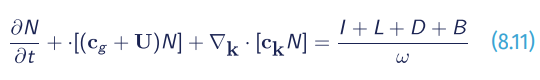
where F(ω,k) is the wave energy density spectrum, ω is intrinsic (from the frame of reference relative to any local current) radian frequency, k is wavenumber (bold symbols signify vector properties). In the linear case, temporal and spatial scales of the waves are linked through the dispersion relationship (see Eq. 8.2).
The left-hand side of Eq. 8.11 represents time/space evolution of the wave action density because of the energy source terms on the right. On the left, cg is group velocity, ck means the spectral advection velocity, U is the current speed, and we note that c =ω/k is phase speed of the waves. ∇ here is the horizontal divergence operator, and ∇k is such an operator in spectral space.
On the right, source terms are physically represented by wind energy input from the wind, I; nonlinear interactions of various orders within the wave spectrum, L, whose role is to redistribute the energy within the spectrum; dissipation energy sinks, D; wave-bottom interaction processes, B; and more sources are possible in specific circumstances. Note that all the source terms, as well as the group and advection velocities, and the advection current are spectra themselves. Please refer to Cavaleri et al. (2007) for further details.
Among the source functions, L is a conservative term, i.e. its integral is zero, but the other integrals define energy fluxes in and out the wave system:
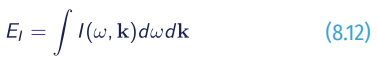
is the total flux of energy from the wind to the waves. Note that, depending on the relative speed of wind U10 and wave speeds c(ω,k)=ω / k, contributions to the total flux can be both positive (from the wind to the waves if U10>c) and negative (from the waves to the wind if U10>c). In the tropics, for example, where the wave climate is dominated by swells produced at high latitudes, the local winds are typically light and therefore the wind climate can be actually dominated by wave-induced winds (Hanley et al., 2010).
It should be noted that the energy input to the waves is generally accepted as a purely atmospheric exchange. In principle, however, energy input from the ocean side to the surface waves of scales accommodated in Eq. 8.11 is perceivable. For example, upper-ocean currents, tides, or internal waves can provide such dynamics. Given the amount of energy stored in the ocean movements, this could have large impacts on surface wave fields, even if localised, but it is fair to say that it has not been considered by the wave-ocean modelling community in practical terms.
Integrating the momentum-input spectrum gives the total momentum flux:
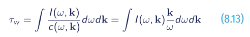
which is an important measure of wind-wave interactions (Tsagareli et al., 2010). Together with the tangential viscous stress τv it forms the total wind stress at the ocean surface
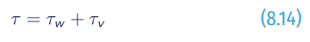
and this stress is known independently (usually through empirical parameterisations of the so-called drag coefficient) and thus can be used as a constraint or for validation of the wind input term I. On the other hand, the total stress is often the main, if not the only property which expresses dynamic exchanges in large-scale air-sea models. Apart from situations of light winds, the wave-induced form drag (Eq. 8.12) provides a dominant contribution to this total stress (Kudryavtsev et al., 2001) and thus, if the wave-model physics is well defined and validated, such models can provide explicit rather than empirical estimates of fluxes for general circulation models if those are appropriately coupled with wave models.
The dissipation function D has a similar meaning in the context of wave-ocean dynamic exchanges, but with some essential distinctions. First, the integral
is the total flux of energy out of the wave field. The energy passed to the ocean is largely spent on generating turbulence near the surface and on work against buoyancy forces acting on bubbles injected during the wave breaking.
Unlike the input, however, which only occurs on the air side of the interface, the loss (8.15) can go both to the ocean below and to the atmosphere above the ocean surface. Numerical simulations of Iafrati et al. (2013) showed that up to 80% of wave energy due to breaking can be actually dissipated through the atmospheric turbulence.
The momentum-loss integral of dissipation function gives the so-called radiation stress:
which is presumed to be going to the currents (although some of it may in fact be going back to the wind, or to the bottom in shallow areas). In the present wave models, radiation stress is parameterized in terms of wave-height difference along the propagation direction. Obviously, such parameterization does describe the energy dissipation, and can then be used to estimate the momentum loss, but only in the areas where dissipation (Eq. 8.14) is much larger than the energy input (Eq. 8.14), i.e. usually in shallow waters. In deep water, the mean wave height is not a proxy for the energy loss. In fact, it may grow under wind action or not change if this action is balanced by the whitecapping dissipation, but the integral (Eq. 8.16) and hence the radiation stress is not zero.
Wave-ocean-bottom interactions in infinite depths, depicted by term B in Eq. 8.11, are very rich. Finite depths are characterised by the condition of kd~1 (wavelength is comparable with the water depth d), and shallow non-dispersive environments by kd<<1. Dispersive-wave nonlinear dynamics slowdown in finite and shallow depths, weaken or cease, but other nonlinear behaviours come into existence.
Wave exchanges with the bottom include bottom friction, formation of ripples, sediment suspension and transport if the sea bed is sandy, generation of bottom waves if the bottom is muddy, and percolation. Long-shore, cross-shore, and rip currents result from radiation stresses (Eq. 8.15), infragravity waves are produced by combined action of wave breaking and nonlinear wave groups, which can be subsequently reflected back to the deep ocean or trapped by coastal bays.
An example of this deep-water approach is the WAM (Hasselmann et al.,1988), perhaps the first one proposed as third-generation model, able to explicitly represent all the physics relevant for the development of the sea state in two dimensions, such as wind generation, whitecapping, quadruplet wave-wave interactions, and bottom dissipation. This modes is mainly forced by a two-dimensional ocean wave spectrum that develops freely with no constraints on the spectral shape, so that: a) a transfer source function of the same degree of freedom as the spectrum itself need to be developed; and b) the energy balance had to be closed by defining the dissipation source function. Hasselmann et al., (1985) and Komen et al., (1984) were employed to deal with these aspects, respectively. The dissipation was selected in order to replicate the observed fetch-limited wave growth and the fully developed Pierson-Moskowitz spectrum (WAMDI group, 1988).
Constant improvements and updates have led to a third-generation WAM model. A third-generation wave model explicitly represents all the physics relevant to the development of the sea state in two dimensions. Numerical solutions of the momentum balance of air flow over growing surface gravity waves have been presented in a series of studies by Janssen et al. (1989), and Janssen (1991). The main conclusion was that the growth rate of the waves generated by wind depends on the ratio of friction velocity and phase speed and on several additional factors, such as the atmospheric density stratification, wind gustiness, and wave age. This work has also introduced the surface stress dependency with the sea state, and the feedback of wave-induced stress on the wind profile in the atmospheric boundary layer.
WAM is an Eulerian phase-averaged model. Designed as a deep-water model, it can be used to predict directional spectra and wave properties (significant wave height, mean wave direction and frequency, swell wave height). The model can be used in finite depth as well by introducing bottom dissipation source function and refraction. The model runs on a spherical latitude-longitude grid.
The first WAVEWATCH model was developed at TU Delft (Tolman, 1989; Tolman 2014), followed by the NASA Goddard Space Flight Centre in 1992. Recently, WAVEWATCH III was presented as a worldwide used and full-spectral third-generation wind-wave model. It was developed at NOAA/NCEP and it is based on the first WAM model’s principles. This latest version includes many improvements in the governing equations, model structure, numerical schemes, and physical parameterizations. The model solves the random phase spectral action density balance equation for wavenumber-direction spectra. The medium properties, namely the water depth and current properties, as well as the wave field, vary in time and space in scales much larger than a single wave. WAVEWATCH is an open-source model that is freely available 🔗3, including the whole source code and all documentation.
The discretization of the wave energy spectra in all directions is achieved by using a constant directional increment and a spatially varying wavenumber grid, which corresponds to an invariant logarithmic intrinsic frequency. In order to achieve high accuracy, both first order and third order schemes are available for wave propagation. For the integration of source terms in time, a semi-implicit scheme is used similar to that used in WAM, which includes a dynamically adjusted time stepping algorithm.
Following the work of Battjes and Janssen (1978), WAM and WAVEWATCH III models have been upgraded to account for the dissipation by wave breaking induced by depth in the surf zone. However, wave models still have difficulties with strong three-wave interactions that occur in finite-depth and shallow waters. That has led to simplified empirical calculations with large errors, especially for complex wave trains with multi-model spectra. In addition, both models lack of diffraction processes, which implies that only open coastal zones could be solved accurately, plus only linear behaviour of wave propagation could be assessed and non-linear corrections to linear wave should be imposed, by triad and quadruplet wave-wave interactions in shallow waters, where the waves break (Booij et al., 1999).
8.4.1.2
Shallow water
Spectral models
For shallow water domains and wave propagation (Eckart, 1952), the SWAN model could be a good choice. This also is a third-generation wave model developed at the Delft University of Technology, with the purpose of obtaining realistic estimates of wave parameters in coastal areas, lakes, and estuaries from given wind, bottom, and current conditions. The SWAN model can be also used on any scale relevant for wind-generated surface gravity waves. The model equations are based on the wave action balance equation with sources and sinks.
SWAN has been developed to simulate coastal wave conditions (with friction, breaking, whitecapping, triad, and quadruplet wave-wave interaction). SWAN can be also coupled with previous models such as WAM or WAVEWATCH III, and inherit the boundary conditions. SWAN can provide a computational representation of directional and no directional spectrum at one point, and several spectral and time-dependent parameters of waves, such as significant wave height, peak or mean period, direction, and direction of energy transport. SWAN is a freely available 🔗4 open-source software.
SWAN model is based on the spectral action balance equation, which describes the evolution of the wave spectrum (Booij et al., 1999).
In Cartesian coordinates the evolution of the action density is governed by the following balance equation:
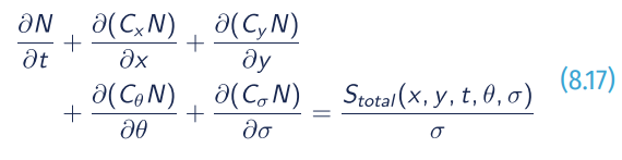
where σ is the wave frequency, θ is the wave direction component, t is the time, x and y the 2D coordinates in space, N the wave action density spectrum defined as:
where E is the wave energy density spectrum; Stotal is the source term and C,S are the wave propagation velocities in space and wavenumber, given by:
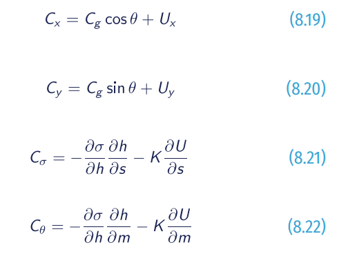
where k is the wavenumber, Cg is the group velocity; s is a coordinate in θ direction and m is a coordinate perpendicular to s; h is the mean water depth and K the wavenumber vector.
The left hand side of Eq. 8.16 corresponds to the kinematic terms, as derivatives for the propagation in space; and are the propagation velocities. The term with the derivative with respect to θ is the refraction term. The term with respect to σ causes a change of frequency. The right hand side is the source term and contains the effects of wind generation, whitecapping, dissipation, bottom friction, surf breaking, and nonlinear wave-wave interaction. This equation is implemented with finite difference schemes in all directions: time, geographic space, and spectral space.
The essential input data to run the model is the bathymetry for a sufficiently large area, the incident wave field, and the wind field. Various general and nested grids can be selected, depending on the availability of high-resolution data and the computational efficiency. Nesting is a very important implementation that can save computational time and increase accuracy. The model is validated with analytical solutions, field observations and experimental measurements, and has shown good agreement (Booij et al., 1999). Moreover, SWAN can operate with unstructured grids as well. Zijlema (2009) presented a method of vertex-based, fully implicit, and finite differences that is designed for unstructured meshes with high variability in geographic resolution. It is useful for complex bottom topographies in shallow areas and irregular shorelines.
SWAN is basically designed for applications in open coastal scale, with no-diffraction effects. That means that the model should be used in areas where variations in wave height are large within a horizontal scale of a few wavelengths.
SWAN organises its output in tables, maps (Figures 8.19 and 8.20) and time series, as well as 1D and 2D spectra, significant wave height and periods, average wave direction and directional spreading, one- and two-dimensional spectral source terms, root-mean-square of the orbital near-bottom motion, dissipation, wave induced force (based on the radiation-stress gradients), set-up, diffraction parameter, etc.
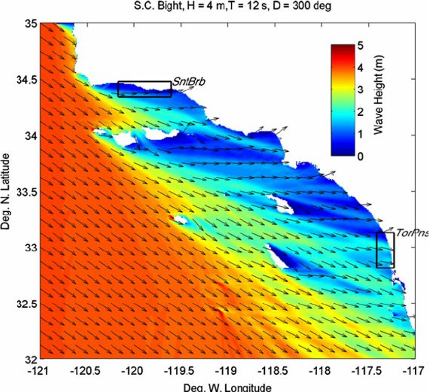
Figure 8.19. Example wave height and direction output from SWAN wave transformation model over the Southern California Bight (source: University of Florida).
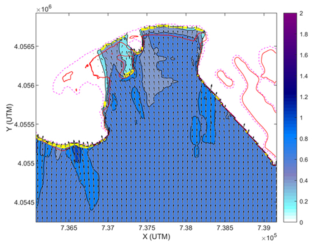
Figure 8.20. Significant wave height propagation map for Los Galeones Beach (Cadiz, Spain) computed with a parabolic Mild-Slope based model (REF-DIFF, OLUCA model) (source: University of Cantabria).
Mild slope equations models
MSE originally developed to describe the propagation of the waves over low gradient seabeds. MSE is commonly used in coastal engineering, since it can account well the effects of simultaneous diffraction and refraction of the waves due to coastlines or structures (Berkhoff, 1972). Mild-slope equations are a type of depth-averaged equation, within a x-y domain (2DH), applied in both deep and shallow waters for monochromatic waves (Lin, 2008).
The equations can be found in various forms, including the effects of wave breaking, nonlinearity of waves, wave-current interactions, and seabed friction. They calculate the wave amplitude or wave height but, if there is a constant water depth, the mild-slope equation reduces to the Helmholtz equation for wave diffraction. First introduced by Berkhoff (1972), the MSE assumed that the wave is linear and the slope is mild, obtaining the following main equation, improved by including the effects of friction dissipation and wave breaking:
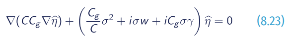
where C is the wave celerity and Cg the group velocity; η̂ is the complex wave surface function; k is the wavenumber; σ is the wave frequency; w is a friction factor and γ is a wave breaking parameter. Friction is then obtained with:
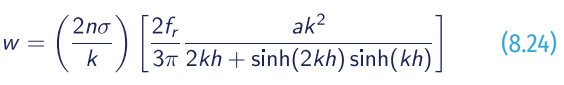
where a is the wave amplitude, and fr is a Reynolds dependent friction coefficient related to the bottom roughness; n is the Manning dissipation coefficient.
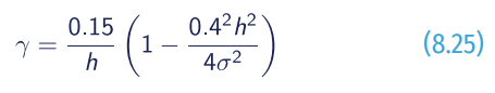
For weave breaking parameter, the following formulation is commonly used:
The original MSE has limitations because it is only applicable to linear waves and on mild bottom geometry. In addition, the equation does not contain energy dissipation, but in recent years there have been numerical advances to include energy dissipation and weakly non-linear waves with steeper bottom slopes. Mild-slope equation has been developed with different formulations that can be described by hyperbolic (Dingemans, 1997), elliptic (Berkhoff, 1972), and parabolic (Lin, 2008) formulation of the mild-slope equation respectively.
The practical application of wave transformation usually requires the simulation of directional random waves; thus, the principle of superposition of different wave frequency components can be applied. In general, MSE models for spectral wave conditions require inputs of the incoming directional random sea at the offshore boundary. The two-dimensional input spectra are discretized into a finite number of frequency and direction wave components.
For the parabolic approach, the evolution of the amplitudes of all the wave components is computed simultaneously. Based on the calculations for all components and assuming a Rayleigh distribution, statistical quantities such as the significant wave height Hs can be calculated at every grid point. Figure 8.20 shows an example for a near-coast wave propagation obtained with a parabolic approximation of the mild slope equation for spectral wave conditions.
When wave reflection becomes relevant for wave propagation and transformation (i.e. within bays, harbours, sheltered areas, etc.), models should be based on the elliptical approximation of the mild-slope equation (Berkhoff, 1972; Madsen and Larsen, 1987; Tsay et al., 1989). This approach allows engineers to obtain the energetic response of reflected (totally or partially) waves, under the penetrating wave action.
Elliptic mild slope models solve the extended mild-slope equation to reproduce the main processes that control dynamics of waves when approaching coastal areas and entering into harbours (Figure 8.21): geometric refraction, shoaling, diffraction by obstacles, and full or partial reflection. Radiation conditions and free infinite outflow conditions are also available in the model. It also considers the complete spectral frequency distribution and the directional spreading of the wave energy spectrum.
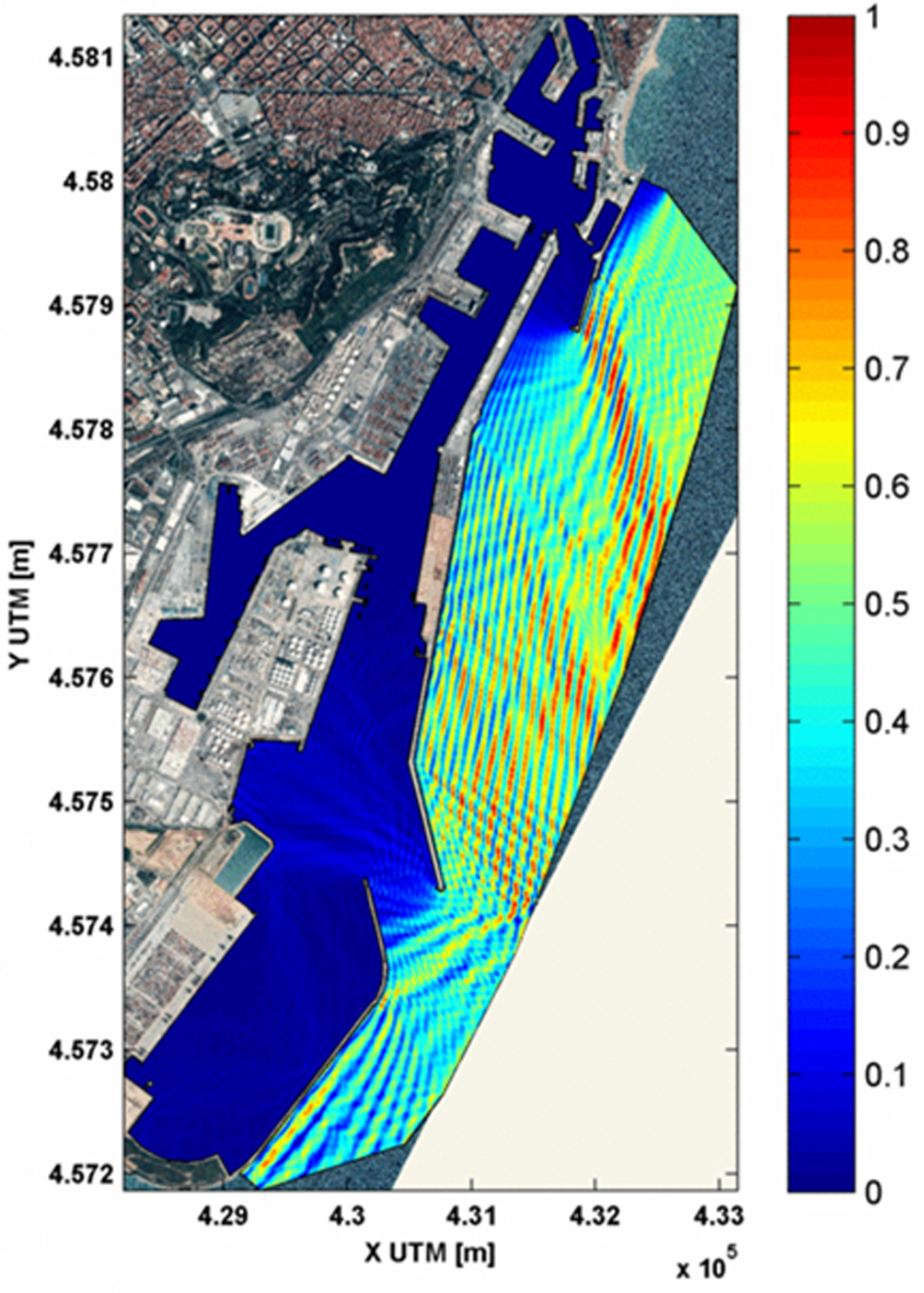
Figure 8.21. Significant wave height map within Barcelona Port computed with an elliptic Mild-Slope based model (MSP model) (source: University of Cantabria and Puertos del Estado).
In addition to the above mechanisms, nonlinear waves may be simulated by incorporating amplitude-dependent wave dispersion, which has been demonstrated to be important in certain situations (Kirby and Dalrymple, 1983).
This practical approach for harbour agitation and wave propagation can be assessed with the following, among others, commercial and non-commercial models: CGWAVE; ARTEMIS MIKE21; PHAROS, and MSP.
Phase resolving models (SWE, NSWE, and Boussinesq)
The Shallow Water Equations (SWE) are applied when water waves enter very shallow domains. Particles move basically horizontally and the vertical accelerations are negligible.
In this case, the propagation of the wave can be described by the SWE (Holthuijsen, 2007). These equations are derived from averaging the depth of the Navier-Stokes equations (NSE) assuming that the horizontal length scale is much greater than the vertical. The profile is uniform in depth and the vertical components very small. Using the conservation of mass, it can be shown that the vertical velocity is small, while using the momentum equation the vertical pressure gradients are hydrostatic. Therefore, the velocity profile is uniform in depth and the vertical components very small, and this is the reason for which SWE are also known as “long-wave equations”, given that they can be applied only to waves which are much larger to the bottom depth.
In the case of ignoring the Coriolis force, the frictional and viscous forces, the formulas of SWE are:
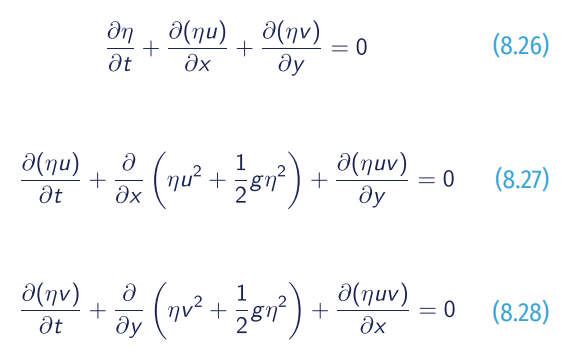
Equation 8.26 is derived from mass conservation and Eqq. 8.27 and 8.28 from momentum conservation, where η is the total fluid column height, (u,v) - a 2D vector - is the fluid’s horizontal velocity in the xy 2D domain.
To represent the ocean waves frequencies and physical behaviour, an improvement within the original SWE is needed, including the non-linearity terms and dispersive functions. The solution for this is the NSWE, as a non-hydrostatic waveflow solution model. It can be used for predicting transformation of dispersive surface waves from offshore to the beach, solving the surf zone and swash zone dynamics, wave propagation and agitation in bays and harbours, and rapidly varied shallow water flows typically found in coastal flooding (e.g. dike breaks, tsunamis and flood waves, density driven flows in coastal waters), as well as large-scale ocean circulation, tides and storm surges (typically solved by the original SWE models).
Main governing equation considers a 2DH wave motion over a domain represented in a Cartesian coordinate system (x,y). The depth-averaged, non-hydrostatic, free-surface flow can be described by the NSWE and comprise the conservation of mass and momentum. These equations are given by:
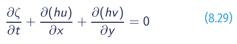
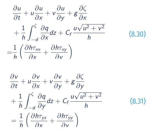
where t is the time; ζ is the free surface elevation, d is the water depth and h=d+ζ, u and v are depth-averaged flow velocities, q is the non-hydrostatic pressure, g the gravitational acceleration, Cf the bottom friction coefficient, and the group of τ are the horizontal turbulent stress terms.
The SWASH (Zijlema et al., 2011) is one of the latest worldwide available 🔗5 NSWE models. It is a numerical tool for simulating unsteady, non-hydrostatic, free-surface, rotational flow, and transport phenomena in coastal waters as driven by waves, tides, buoyancy, and wind forces. It provides a general basis for describing wave transformations from deep water to the beach, port or harbour, as well as complex changes to rapidly varied flows, and density driven flows in coastal seas, estuaries, lakes, and rivers. SWASH is an efficient and robust model that allows the application of a wide range of time and space scales of surface waves and shallow water flows in complex environments (Figure 8.22). The model can be also employed to resolve the dynamics of wave transformation, buoyancy flow, and turbulent exchange of momentum, salinity, heat, and suspended sediment in shallow seas, coastal waters, estuaries, reefs, rivers, and lakes.
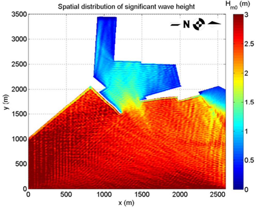
Figure 8.22. Results from the SWASH model for the wave condition at Limassol Port (Cyprus) (from Van der Ven et al., 2018).
SWASH may be run in depth-averaged mode or multi-layered mode in which the computational domain is divided into a fixed number of vertical terrain-following layers. SWASH improves its frequency dispersion by increasing the number of layers rather than increasing the order of derivatives of the dependent variables like Boussinesq-type wave models do.
BE can be applied as an alternative to NSWEs as the region between deep and shallow waters can be also well described by the Boussinesq model. In BE models, the horizontal component of the velocity is assumed to be constant in the water column and the vertical component of the velocity varies almost linearly over depth (2DH hypothesis). Essentially, these equations are the shallow-water equations with corrections for the vertical acceleration, and third order derivatives are the result of the Laplace equation forcing the vertical velocity of the velocity potential function to be expressed in terms of the horizontal velocity distribution. These equations can be readily expanded into two horizontal dimensions.
Researchers have introduced many different implementations of the Boussinesq equations, creating Boussinesq-type models to be applied for propagation in deep water and the process of wave-breaking (Brocchini, 2013). A vast majority of Boussinesq equations models (for fully non-linear approach) can be presented as follows:
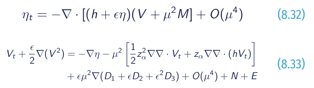
with
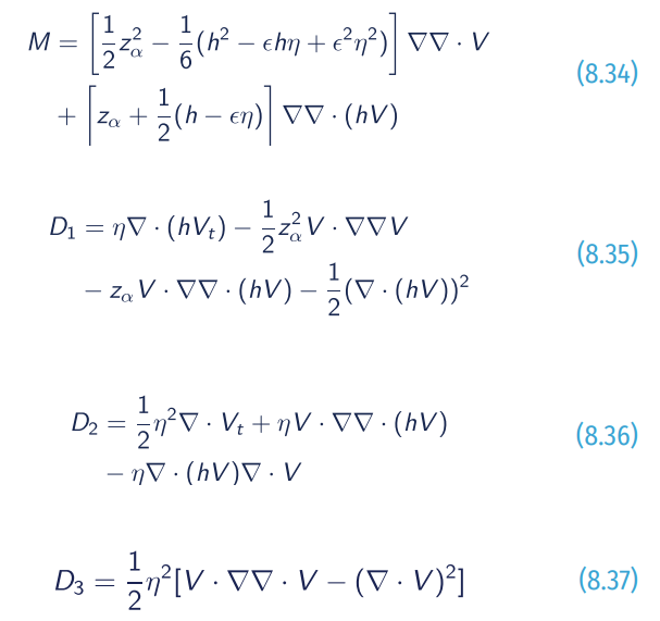
where index of t denotes time; h is the equilibrium depth; η is the free-surface elevation, V is the horizontal velocity, and ∇ is the 2DH gradient operator. N and E respectively represent bottom drag and diffusion (artificial).
On the other hand, a similar family of equations exist and are applied in the region between deep and shallow waters; the Boussinesq equation-based model. For this approach, the main hypothesis is that the horizontal component of the velocity is assumed to be constant in the water column, and the vertical component of the velocity varies almost linearly over depth.
One of the most complete Boussinesq models, the fully nonlinear Boussinesq wave model (FUNWAVE) in its TVD version known as FUNWAVE-TVD model (Fengyan, et al., 2012), was developed at the Centre for Applied Coastal Research at the University of Delaware (USA). It includes several enhancements: i) a more complete set of fully nonlinear Boussinesq equations; ii) a MUSCLE-TVD finite volume scheme together with adaptive Runge Kutta time stepping; iii) shock-capturing wave breaking scheme, iv) wetting-drying moving boundary condition with HLL construction method for the scheme; and v) code parallelization using MPI method. The development of the FUNWAVE-TVD was prompted by the need to model tsunami waves in regional and coastal scale, coastal inundation, and wave propagation at basin scale (Figure 8.23). FUNWAVE is an open-source model available to the public 🔗6.
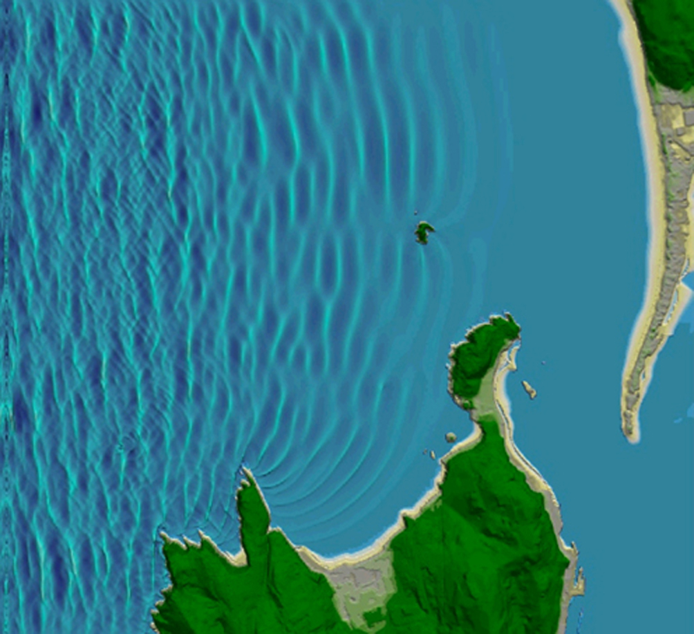
Figure 8.23. Free surface snapshot from the FUNWAVE-TVD applied in Sardinero Beach and Santander Bay (Spain) outer and inner zone (source: University of Cantabria).
Numerical solutions of Boussinesq equations can be significantly corrupted if truncation errors, arising from the differencing of the leading order wave equation terms, are allowed to grow in size and become comparable to the terms describing the weak dispersion effects. All errors involved in solving the underlying nonlinear SWE are reduced to 4th order in grid spacing and time step size. Due to non-linear interaction in the model, higher harmonic waves will be generated as the program runs. These super harmonic waves could have very short wavelengths and the classic Boussinesq model is not valid. For this reason, a numerical filter suggested by Shapiro (1970) can be used.
In summary, both Boussinesq and NSWEs modelling approaches are the preferred solutions in their respective physical regions: Boussinesq where nonlinearity and dispersion are both significant, typically prior to breaking; and NSWE where nonlinearity predominates, from the mid-surf to inner surf zone shoreward, although it should be noted that there can be a significant overlap of these regions. Therefore, the NSWE models, which work well from the surf zone shoreward and naturally model wave breaking and the moving shoreline, find their main weakness in the absence of frequency dispersion, so that in deeper water waves will propagate incorrectly at the shallow water wave speed and, sooner or later, break again, which is not usual and correct in this region.
Two- and three-dimensions wave structure interaction model
CFD utilises numerical approaches to examine fluid flows, heat transfer and chemical reactions. Therefore, within wave propagation and structure interaction problems, the CFD term mainly refers to computer codes that solve the fully nonlinear Navier-Stokes equations in all three dimensions (3D).
CFD is then a state-of-the-art techniques for industrial and research applications, although its often high computation cost demands the use of high-performance computers. Within the wave propagation and wave structure interaction field, two of the most used CFD programs are: IH2VOF (two-dimension approach, derived from COBRAS original model) and OpenFOAM (three-dimension approach); these two codes are also well validated for many marine and ocean engineering applications.
As a classic Eulerian approach, both models are based on the RANS equations. These equations represent the continuum properties of the flow. By averaging the Navier-Stokes equations, more recent VARANS equations are obtained. The VARANS equations can have different terms, depending on the assumptions applied; for example, they include a k-ω turbulence model closure within the porous media, which make them the most suitable formulation for coastal engineering as the advantages of VARANS equations are numerous. The solving process yields very detailed solutions, both in time and space. Pressure and velocity fields are obtained cell-wise, even inside the porous zones, so that the whole three-dimensional flow structure is solved. Furthermore, non-linearity is inherent to the equations, and therefore all the complex interactions among the different processes are also taken into consideration. Finally, the effects of turbulence within the porous zones can be also easily incorporated with closure models.
IH2VOF model (Lara et al., 2006) solves 2D RANS equations for the oscillatory fluid and VARANS equations for the porous media. This 2D model can simulate the most relevant hydrodynamic near-field processes that take place in the interaction between waves and low-crested breakwaters. It considers wave reflection, transmission, overtopping, and breaking due to transient nonlinear waves, including turbulence in the fluid domain and in the permeable regions for any kind of geometry and number of layers. This model is highly validated, with different wave conditions and breakwater configurations, achieving a high degree of agreement with all the studied magnitudes, free surface displacement, pressure inside the porous structure, and velocity field.
IH2VOF is based on the decomposition of the instantaneous velocity and pressure fields into mean and turbulent components, the κ-ε equations for the turbulent kinetic energy κ, and its dissipation rate ε. This permits the simulation of any kind of coastal structure (e.g. rubble mound, vertical or mixed breakwaters). The free surface movement is tracked by the volume of fluid (VOF) method for one phase only, water and void. In order to replicate solid bodies immersed in the mesh instead of treating them as sawtooth shape, the model uses a cutting cell method. The main purpose of this technique is to use an orthogonal structured mesh in the simulations to save computational cost.
IH2VOF includes a complete set of wave generation boundary conditions, which cover most water depth ranges. These include a Dirichlet boundary condition and a moving boundary method, which are linked with an active wave absorption system to avoid an increase of the mean water level and the agitation. An internal source function can be also used to generate waves, but it has to be linked with a dissipation zone.
The RANS equations (clear fluid region) are redefined as follows:
Generally, IH2VOF application is within a detailed incident-wave and structure interaction (rubble-mound breakwaters, vertical structures and beaches), taking into account a realistic wave breaking and porous media interaction (see Figure 8.24).
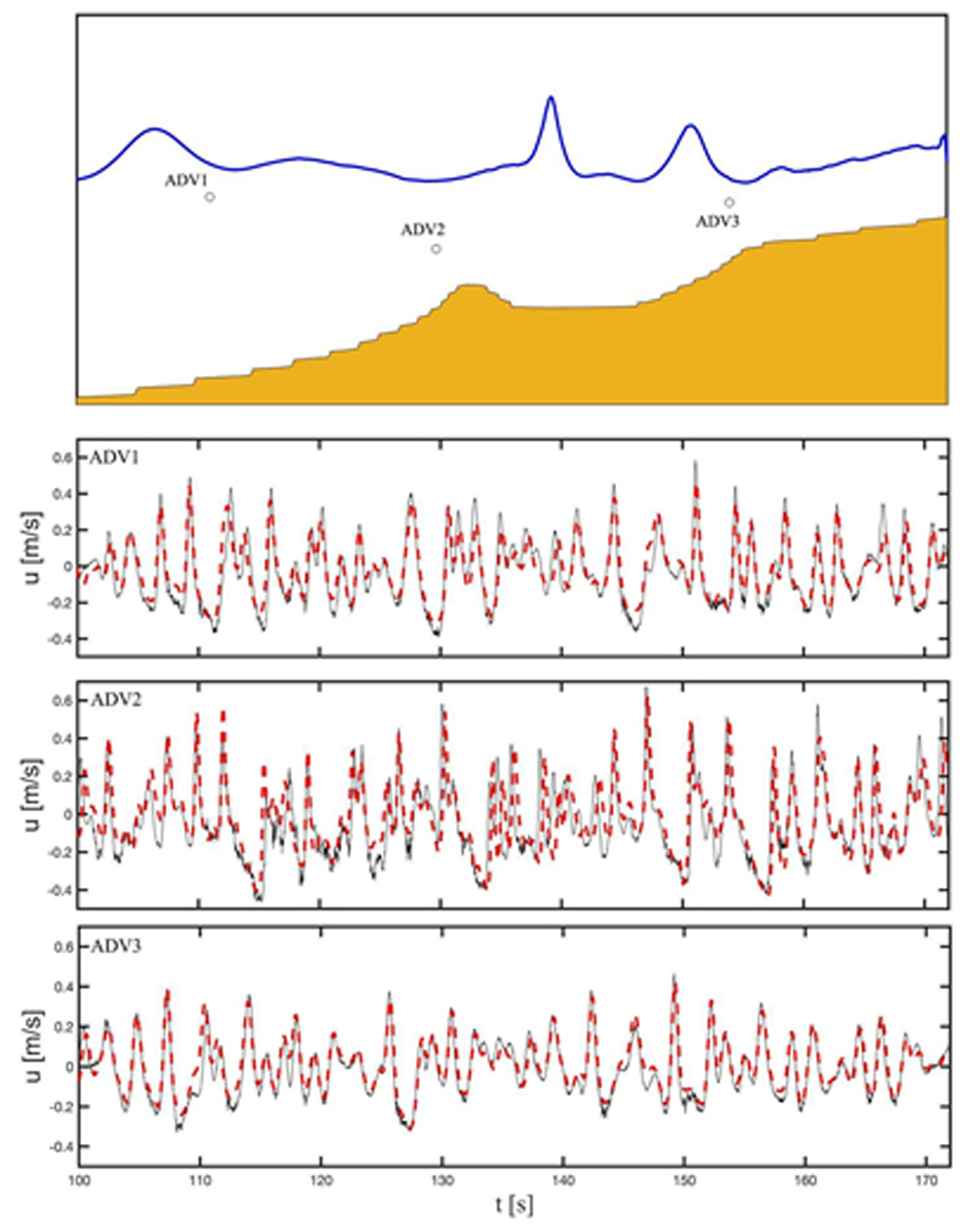
Figure 8.24. Irregular wave propagation towards a real profile beach. Free surface snapshot and wave velocity validation against field measurements (source: National University of Mexico).
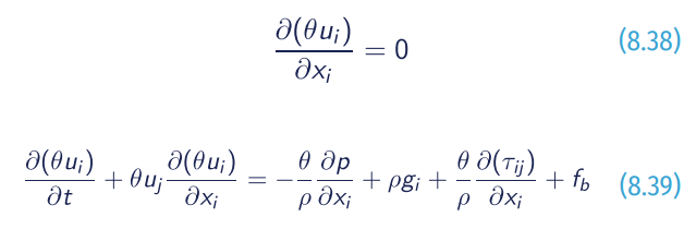
The general VARANS equations include conservation of mass (8.39), conservation of momentum (8.40), and the VOF function advection equation (8.41) as follows:
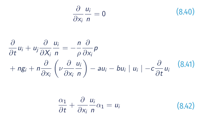
where u is the extended averaged Darcy velocity; n is the porosity (volume of voids over the total volume); ρ is the density; p is the pressure; g is the acceleration of gravity; ν is the kinematic viscosity, and α1 is the VOF function indicator (quantity of water per unit of volume at each cell).
The OpenFOAM (Higuera et al., 2014a and 2014b) is an extensive software package that has been widely used in industrial and academic applications. It is freely distributed 🔗7 as an open source CFD Toolbox, and it includes a broad range of features. IHFOAM 2.0 is an extension of the original software for coastal applications, newly developed with a three-dimensional numerical two-phase flow solver, specially designed to simulate coastal, offshore, and hydraulic engineering processes. It contains an advanced multiphysics model, widely used in the industry. A wide collection of boundary conditions, which handle wave generation and active absorption at the boundaries with a high practical application to coastal and harbour engineering (Figure 8.25), makes IHFOAM 2.0 different from the rest of solvers. Maza et al. (2016) have studied and proposed natural-based solutions for coastal protections using IHFOAM.
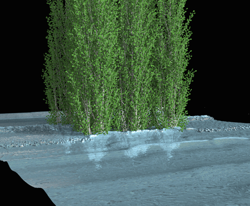
Figure 8.25. Free surface snapshot of irregular wave interacting with a natural-based protection (a tree patch) calculated with IHFOAM 2.0 (source: University of Cantabria).
8.4.2
Discretization methods
Various discretization methods are used in water wave solving problems, a brief description for each of them is presented below (for additional references see Sections 5.4.2.4 and 7.2.3.5):
- FDM. Maybe the most used and simplest ways to solve numerically partial differential equations (PDEs). The method establishes the value of the flow variable at a given point based on the number of neighbour points. The numerical domain forms a grid. The governing equations of the fluid are considered in their differential form at each point in the domain, so that the solution is solved by replacing the partial derivatives with approximations by means of the nodal values of the functions. This method is recommended for structured grids and low-order equation schemes.
- FEM for the solution of PDEs employs variational methods to minimise the error of the approximated solution, similarly to the Galerkin method. FEM was used in structural mechanics but this technique developed for computational fluid dynamics applications being introduced to common wave propagation and agitations models. FEM technique, similarly to the FDM, is based on the concept of subdividing a continuum computational domain into elements, forming a grid of triangular or quadrilateral unstructured elements or curved cells (Figure 8.26). Therefore, the method can handle problems with great geometric complexity, such as harbour perimeter definition, concentration of nodes at relevant parts of the domain, etc.
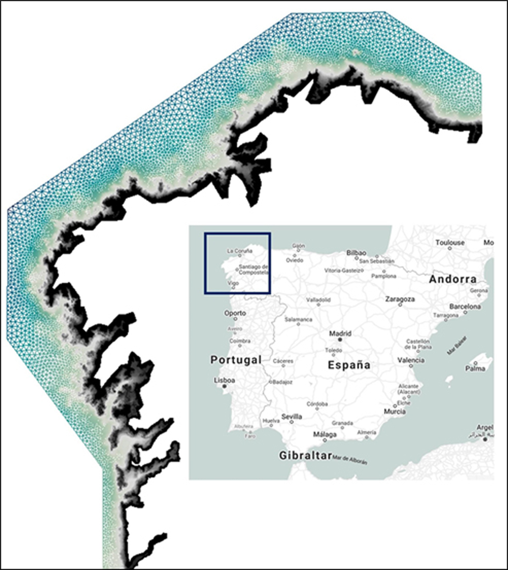
Figure 8.26. Finite Element Metod (FEM) based on irregular sized triangles applied to Galicia (Spain) for SWAN model (source: University of Cantabria).
FEM used variational methods, which in practice means that the solution is assumed to have a prescribed form and to belong to a function space. The function space is built by varying functions, such as linear and quadratic. The varying functions connect the nodal points, which can be the vertices, mid-side points, mid-element points, etc., of the elements. As a result, the geometric representation of the domain plays a crucial role in the outcome of the numerical simulation. The original PDEs are not solved by the FEM. Instead, the solution is approximated locally by an integral form of the PDEs. The integral of the inner product of the residual and the weight functions are constructed. The integral is set to zero and trial functions are used to minimise the residual. The most general integral form is obtained from a weighted residual formulation. The process eliminates all the spatial derivatives from the PDEs and, therefore, differential type boundary conditions for transient problems and algebraic type boundary conditions for steady state problems can be considered, hence the differential equations become algebraic. Only one equation is solved per grid node, which has one variable as unknown. The same variable is also unknown at the neighbouring cells.
- FVM solves PDEs by transforming them to algebraic equations around a control volume (subdivisions of the computational domain). The variables are calculated at the centre of each control volume. General interpolation methods are used to derive the values of the variables at the surfaces of the control volume considering the neighbour control volumes as well. The FVM has two major advantages: i) it is able to accommodate any type of grid, making it applicable for domains of high complexity; and ii) it is conservative by definition, since the control volumes that share a boundary have the same surface integrals, describing the convective and diffusive fluxes. FVMs are very popular in the numerical wave propagation community, succeeding in free surface flow simulations, especially when highly nonlinear processes are involved, such as wave breaking
References
Álvarez-Fanjul, E., García-Sotillo, M., Pérez Gómez, B., García Valdecasas, J. M., Pérez Rubio, S., Rodríguez Dapena, A., et al. (2018). Operational oceanography at the service of the ports. In: “New Frontiers in Operational Oceanography”, Editors: E. Chassignet, A. Pascual, J. Tintoré, and J. Verron (Cambridge: GODAE OceanView), 729-736, https://doi.org/10.17125/gov2018.ch27
Alves, J.-H.G.M., Wittmann, P., Sestak, M., Schauer, J., Stripling, S., Bernier, N.B., Mclean, J., Chao, Y., Chawla, A., Tolman, H., Nelson, G., and Klotz, S. (2013). The NCEP–FNMOC combined wave ensemble product: expanding benefits of inter-agency probabilistic forecasts to the oceanic environment. Bulletin of the American Meteorological Society, 94(12), 1893-1905, https://doi.org/10.1175/BAMS-D-12-00032.1
Aouf, L., Hauser, D., Law-Chune, S., Chapron, B., Dalphinet, A., and Tourain, C. (2021). New directional wave observations from CFOSAT: impact on ocean/wave coupling in the Southern Ocean. EGU General Assembly 2021, online, 19-30 Apr 2021, EGU21-7412, https://doi.org/10.5194/egusphere-egu21-7412
Aouf, L., Lefèvre, J., and Hauser, D. (2006). Assimilation of Directional Wave Spectra in the Wave Model WAM: An Impact Study from Synthetic Observations in Preparation for the SWIMSAT Satellite Mission. Journal of Atmospheric and Oceanic Technology, 23(3), 448-463, https://doi.org/10.1175/JTECH1861.1
Aouf, L., Danièle, H., Céline, T., Bertrand, C. (2018). On the Assimilation of Multi-Source of Directional Wave Spectra from Sentinel-1A and 1B, and CFOSAT in the Wave Model MFWAM: Toward an Operational Use in CMEMS-MFC. IGARSS 2018 - 2018 IEEE International Geoscience and Remote Sensing Symposium, 2018, pp. 5663-5666, doi:10.1109/IGARSS.2018.8517731
Ardhuin, F., Otero, M., Merrifield, S., Grouazel, A., and Terril, E. (2020). Ice breakup controls dissipation of wind waves across Southern Ocean sea ice. Geophysical Research Letters, 47, e2020GL087699. https://doi.org/10.1029/2020GL087699
Ardhuin, F., Rogers, E., Babanin, A., Filipot, J.-F., Magne, R., Roland, A., van der Westhuysen, A., Queffeulou, P., Lefevre, J.-M., Aouf, L., Collard, F. (2010). Semi-empirical dissipation source functions for ocean waves. Part I: definitions, calibration and validations. Journal of Physical Oceanography, 40, 1917-1941, https://doi.org/10.1175/2010JPO4324.1
Babanin, A.V. (2011). Breaking and Dissipation of Ocean Surface Waves. Cambridge University Press, 480 p.
Babanin, A.V. (2018). Change of regime of air-sea dynamics in extreme Metocean conditions. Proceedings of the ASME 2018 37th International Conference on Ocean, Offshore and Arctic Engineering OMAE2018, June 17-22, 2018, Madrid, Spain, paper 77484, 6 p.
Babanin, A.V., Onorato, M., and Qiao, F. (2012). Surface waves and wave-coupled effects in lower atmosphere and upper ocean. Journal of Geophysical Research: Ocean, 117(C11), https://doi.org/10.1029/2012JC007932
Babanin, A.V., van der Westhuysen, A., Chalikov, D., and Rogers, W.E. (2017). Advanced wave modelling including wave-current interaction. In “The Sea: The Science of Ocean Prediction”, Eds. Nadia Pinardi, Pierre F. J. Lermusiaux, Kenneth H. Brink and Ruth Preller, Journal of Marine Research, 75, 239-262.
Barstow, S., Mørk, G., Lønseth, L., and Schjølberg, P.. (2004). Use of satellite wave data in the world waves project. Gayana (Concepción), 68(2, Supl.TIProc), 40-47, http://dx.doi.org/10.4067/S0717-65382004000200007
Battjes, J.A., and Janssen, P.A.E..M. (1978). Energy Loss and Setup Due to Breaking in Random Waves. Proceedings of 16th Coastal Engineering Conference, Hamburg, Germany, 569-587.
Bauer, E., Hasselmann, S., Hasselmann, K. and Graber, H. C. (1992). Validation and assimilation of Seasat altimeter wave heights using the WAM wave model. Journal of Geophysical Research: Ocean, C97, 12671-12682, https://doi.org/10.1029/92JC01056
Berkhoff, J. C. (1972). Computation of combined refraction-diffraction. 13th International Conference on Coastal Engineering, (pp. 471-490). ASCE.
Beven J. (2019). Hurricane Pablo tropical cyclone report, NHC-NOAA.
Bidlot J. R. (2016). Twenty-one years of wave forecast verification. ECMWF Newsletter, 150, 2016.
Booij, N., Ris, R., and Holthuijsen, Leo. (1999). A third-generation wave model for coastal regions, Part I, Model description and validation. Journal of Geophysical Research: Ocean, 104. 7649-7656, https://doi.org/10.1029/98JC02622
Breivik, L-A., Reistad, M., Schyberg, H., Sunde, J., Krogstad, H. E., and Johnsen, H. (1998). Assimilation of ERS SAR wave spectra in an operational wave model. Journal of Geophysical Research: Ocean, 103, 7887- 7900, https://doi.org/10.1029/97JC02728
Breivik, Ø., Gusdal, Y., Furevik, B.R., Aarnes, O.J., Reistand, M. (2009). Nearshore wave forecasting and hindcasting by dynamical and statistical downscaling. Journal of Marine Systems, 78, S235-S243, https://doi.org/10.1016/j.jmarsys.2009.01.025
Breivik, Ø., Mogensen, K., Bidlot, J.-R., Balmaseda, M. A., and Janssen, P. A. E. M. (2015), Surface wave effects in the NEMO ocean model: Forced and coupled experiments. Journal of Geophysical Research: Ocean, 120, 2973-2992, https://doi.org/10.1002/2014JC010565
Brocchini, M. (2013). A reasoned overview on Boussinesq-type models: the interplay between physics, mathematics and numerics. Proceedings of the Royal Society A Mathematical, Physics and Engineering Science, 469, https://doi.org/10.1098/rspa.2013.0496
Browne, M., Castelle, B., Strauss, D., Tomlinson, R., Blumenstein, M., Lane, C. (2007). Near-shore swell estimation from a global wind–wave model: spectral process, linear and artificial neural network models. Coastal Engineering, 54, 445-460, https://doi.org/10.1016/j.coastaleng.2006.11.007
Bunney, C., and Saulter, A. (2015). An ensemble forecast system for prediction of Atlantic-UK wind waves. Ocean Modelling, 96(1), 103-116, doi: 10.1016/j.ocemod.2015.07.005
Dean, R. G., Dalrymple, R. A. (1991). Water wave mechanics for engineers and scientists (Advanced series on ocean engineering - Volume 2), Singapore World Scientific Publishing.
Camus, P., Mendez, F., Medina, R. (2011). A hybrid efficient method to downscale wave climate to coastal areas. Coastal Engineering, 58(9), 851-862, https://doi.org/10.1016/j.coastaleng.2011.05.007
Camus, P., Mendez, F.J., Medina, R., Tomas, A., Izaguirre, C. (2013). High resolution downscaled ocean waves (DOW) reanalysis in coastal areas. Coastal Engineering, 72, 56-68, https://doi.org/10.1016/j.coastaleng.2012.09.002
Cavaleri, L., Alves, J.-H.G.M., Ardhuin, F., Babanin, A., Banner, M., Belibassakis, K., Benoit, M., Donelan, M., Groeneweg, J., Herbers, T.H.C., Hwang, P., Janssen, P.A.E.M., Janssen, T., Lavrenov, I.V., Magne, R., Monbaliu, J., Onorato, M., Polnikov, V., Resio, D., Rogers, W.E., Sheremet, A., McKee Smith, J., Tolman, H.L., van Vledder, G., Wolf, J., Young, I. (2007). Wave modeling - the state of the art. Progress in Oceanography, 75(4), 603-674, https://doi.org/10.1016/j.pocean.2007.05.005
Cavaleri, L., Abdalla, S., Benetazzo, A., Bertotti, L., Bidlot, J.-R., Breivik, Ø., Carniel, S., Jensen, R.E., Portilla-Yandun, J., Rogers, W.E., Roland, A., Sanchez-Arcilla, A., Smith, J.M., Staneva, J., Toledo, Y., van Vledder, G.Ph., and van der Westhuysen, A.J. (2018). Wave modelling in coastal and inner seas. Progress in Oceanography, 167, 164-233, https://doi.org/10.1016/j.pocean.2018.03.010
CERC, (1984). Shore Protection Manual. Department of the Army US. Army Corps of Engineers, Washington DC.
Chalikov, D. (2016). Numerical Modeling of Sea Waves. Springer, 330 p.
Chelton, D. B., and McCabe, P. J. (1985). A review of satellite altimeter measurement of sea surface wind speed: with a proposed new algorithm. Journal of Geophysical Research: Oceans, 90(3), 4707-4720, https://doi.org/10.1029/JC090iC03p04707
Chen, H.S. (2006). Ensemble Prediction of Ocean Waves at NCEP. Proceedings of 28th Ocean Engineering Conference, Taiwan.
Climate Change Initiative Coastal Sea Level Team(The).(2020). Coastal sea level anomalies andassociatedtrends from Jason satellite altimetry over 2002-2018. Scientific Data, 7, 357, https://doi.org/10.1038/s41597-020-00694-w
Dean, R. G., and Dalrymple, R. A. (1991). Water wave mechanics for engineers and scientists. In: “Advanced Series on Ocean Engineering: Volume 2” by R.G. Dean and R.A. Dalrymple, World Scientific Publishing Co Pte Ltd, https://doi.org/10.1142/1232
Derkani, M. H., Alberello, A., Nelli, F., Bennetts, L.G., Hessner, K. G., MacHutchon, K., Reichert, L., Aouf, L., Khan, S., Toffoli, A. (2021). Wind, waves, and surface currents in the Southern Ocean: observations from the Antarctic Circumnavigation Expedition. Earth System Science Data, 13, 1189-1209, https://doi.org/10.5194/essd-13-1189-2021
Dingemanns, M. (1997). Waterwave propagation over uneven bottoms. Advanced Series on Ocean Engineering, 13(2), 967.
Donelan, M., Haus, B.K., Reul, N., Plant, W., Stiassnie, M., Graber, H.C., Brown, O., Saltzman, E. (2004). On the limiting aerodynamic roughness of the ocean in very strong winds. Geophysical Research Letters, 31(18), https://doi.org/10.1029/2004GL019460
Durrant, T.H., Woodcock F., and Greenslade, D.J.M. (2009). Consensus forecasts of modelled wave parameters. Weather and Forecasting, 24, 492-503, https://doi.org/10.1175/2008WAF2222143.1
Ebert, E. (2001). Ability of a poor man’s ensemble to predict the probability and distribution of precipitation. Monthly Weather Review,129(10), 2461–2480, https://doi.org/10.1175/1520-0493(2001)129<2461:AOAPMS>2.0.CO;2
Ebert, E.E. (2008). Fuzzy verification of high resolution gridded forecasts: A review and proposed framework. Meteorological Applications, 15, 51-64, https://doi.org/10.1002/met.25
Eckart, C. (1952). The propagation of gravity waves from deep to shallow water. Circular 20, National Bureau of Standards, 165-173.
Edson, J.B., Jampana, V., Weller, R.A., Bigorre, S.P., Plueddemann, A.J., Fairall, C.W., Miller, S.D., Mahrt, L., Vickers, D., and Hersbach, H. (2013). On the exchange of momentum over the open ocean. Journal of Physical Oceanography, 43(8), 1589-1610, https://doi.org/10.1175/JPO-D-12-0173.1
Fengyan, S., Kirby, J. T., Tehranirad, B., Harris, J. C., and Grilli, S. (2012). FUNWAVE-TVD: Fully Nonlinear Boussinesq Wave Model with TVD Solver. Documentation and User’s Manual (Version 2.0). Center for Applied Coastal Research, University of Delaware, Newark, DE. Available at: https://www1.udel.edu/kirby/papers/shi-etal-cacr-11-04-version2.0.pdf
Gaslikova, L., Weisse, R. (2006). Estimating near-shore wave statistics from regional hindcasts using downscaling techniques. Ocean Dynamics, 56, 26-35, https://doi.org/10.1007/s10236-005-0041-2
Greenslade, D.J.M. and Young, I.R. (2004). Background errors in a global wave model determined from altimeter data. Journal of Geophysical Research: Oceans, 109(C9), https://doi.org/10.1029/2004JC002324
González-Marco, D., Sierra, J. P., Ybarra, O. F., Sánchez-Arcilla, A. (2008). Implications of long waves in harbour management: The Gijón port case study. Ocean & Coastal Management, 51(2), 180-201, https://doi.org/10.1016/j.ocecoaman.2007.04.001
Groeneweg, J., Ledden, M., Zijlema, M. (2007). Wave transformation in front of the Dutch Coast. Proceedings of the Coastal Engineering Conference, 552-564, https://doi.org/10.1142/9789812709554_0048
Gulev, S. K., Grigorieva, V., Sterl, A., and Woolf, D. (2003). Assessment of the reliability of wave observations from voluntary observing ships: Insights from the validation of a global wind wave climatology based on voluntary observing ship data. Journal of Geophysical Research: Oceans, 108(C7), https://doi.org/10.1029/2002JC001437
Hanley, K.E., Belcher, S.E., and Sullivan, P.P. (2010). A global climatology of wind-wave interaction. Journal of Physical Oceanography, 40, 1263-1282, https://doi.org/10.1175/2010JPO4377.1
Hanson, J. L., Phillips, O. M. (2001). Automated Analysis of Ocean Surface Directional Wave Spectra. Journal of Atmospheric and Oceanic Technology, 18(2), 277-293, https://doi.org/10.1175/1520-0426(2001)018<0277:AAOOSD>2.0.CO;2
Hansom, J. et al. (2015). Extreme Waves: Causes, Characteristics and Impact on Coastal Environments and Society January 2015. In: “Coastal and Marine Hazards, Risks, and Disasters”, Edition: Hazards and Disasters Series, Elsevier Major Reference Works, Chapter 11: Extreme Waves: Causes, Characteristics and Impact on Coastal Environments and Society. Publisher:; Elsevier; Editors: Ellis, J and Sherman, D. J.
Hasselmann, K. (1962). On the non-linear energy transfer in a gravity-wave spectrum part 1. General theory. Journal of Fluid Mechanics, 12 (4), 481-500.
Hasselmann, K., Barnett, T. P., Bouws, E., Carlson, H., Cartwright, D. E., Enke, K., Ewing, J. A.,Gienapp, H., Hasselmann, D. E., Kruseman, P., Meerburg, A., M¨uller, P., Olbers, D. J., Richter, K., Sell, W. and Walden, H. (1973). Measurements of wind-wave growth and swell decay during the Joint North Sea Wave Project (JONSWAP). Hydraulic Engineering Reports,. Available at: https://repository.tudelft.nl/islandora/object/uuid%3Af204e188-13b9-49d8-a6dc-4fb7c20562fc
Hasselmann, K., Hasselmann, K., Bauer, E., Janssen, P., Komen, G., Bertotti, L., Lionello, P., Guillaume, A., Cardone, V., Greenwood, J., Reistad, M., Zambresky, L., Ewing, J. (1988). The WAM model - a third generation ocean wave prediction model. Journal of Physical Oceanography, 18, 1775-1810.
Hasselmann, S., Hasselmann, K., Allender, J. H., and Barnett, T. P. (1985). Computations and parameterizations of the nonlinear energy transfer in a gravity wave spectrum, II, Parameterizations of the nonlinear energy transfer for application in wave models. Journal of Physical Oceanography, 15, 1378-1391.
Hasselmann, K. (1997). Multi-pattern fingerprint method for detection and attribution of climate change. Climate Dynamics, 13, 601-611, https://doi.org/10.1007/s003820050185
Hasselmann, K., Chapron, B., Aouf, L., Ardhuin, F., Collard, F., Engen, G., Hasselmann, S., Heimbach, P., Janssen, P., Johnsen, H., et al. (2013). The ERS SAR wave mode: A breakthrough in global ocean wave observations. In: “ERS Missions: 20 Years of Observing Earth”, 1st ed.; Fletcher, K., Ed.; European Space Agency: Noordwijk, The Netherlands, 2013; pp. 165-198.
Herman, A., Kaiser, R., Niemeyer, H.D. (2009). Wind-wave variability in shallow tidal sea - spectral modelling combined with neural network methods. Coastal Engineering, 56(7), 759-772, https://doi.org/10.1016/j.coastaleng.2009.02.007
Hersbach H. (2000). Decomposition of the continuous ranked probability score for ensemble prediction systems. Weather and Forecasting, 5(15), 1697-1709, https://doi.org/10.1175/WAF-D-16-0164.1
Hewitt, J. E, Cummings, V. J., Elis, J. I., Funnell, G., Norkko, A., Talley, T.S., Thrush, S.F. (2003). The role of waves in the colonisation of terrestrial sediments deposited in the marine environment. Journal of Experimental Marine Biology and Ecology, 290, 19-47, https://doi.org/10.1016/S0022-0981(03)00051-0
Higuera, P., Lara, L. J., Losada, I.J. (2014a). Three-dimensional interaction of waves and porous coastal structures using OpenFOAM®. Part I: Formulation and validation. Coastal Engineering, 83, 243-258, https://doi.org/10.1016/j.coastaleng.2013.08.010
Higuera, P., Lara, L. J., Losada, I.J. (2014b). Three-dimensional interaction of waves and porous coastal structures using OpenFOAM®. Part II: Application. Coastal Engineering, 83, 259-270, https://doi.org/10.1016/j.coastaleng.2013.09.002
Holthuijsen, L.H. (2007). Waves in Oceanic and Coastal Waters. Cambridge University Press, https://doi.org/10.1017/CBO9780511618536
Iafrati, A., Babanin, A.V., Onorato, M. (2013). Modulational instability, wave breaking and formation of large scale dipoles. Physical Review Letters, 110, 184504, : https://doi.org/10.1103/PhysRevLett.110.184504
Janssen, P.A.E.M (1989). Wave-induced stress and the drag of air flow over sea waves. Journal of Physical Oceanography, 19(6), 745-754, https://doi.org/10.1175/1520-0485(1989)019<0745:WISATD>2.0.CO;2
Janssen, P.A.E.M (1991). Quasi-linear theory of wind wave generation applied to wave forecasting. Journal of Physical Oceanography, 21, 1631-1642.
Janssen, P.A.E.M. (2004). The Interaction of Ocean Waves and Wind. Cambridge University Press, 308 p.
Janssen, P.A.E.M. (2012). Ocean wave effects on the daily cycle in SST. Journal of Geophysical Research: Oceans, 117, C00J32, https://doi.org/10.1029/2012JC007943
Janssen, P.A.E.M., Lionello, P., Reistad, M. and Hollingsworth, A. (1989). Hindcasts and data assimilation studies with the WAM model during the Seasat period. Journal of Geophysical Research: Oceans, C94, 973-993.
Janssen, P.A.E.M., Abdalla, S., Hersbach, H., Bidlot, J.R. (2007). Error estimation of buoy, satellite, and model wave height data. Journal of Atmospheric and Oceanic Technology, 24:1665-1677, https://doi.org/10.1175/JTECH2069.1
Kalra, R., Deo, M.C., Kumar, R., Agarwal, V.K. (2005). Artificial neural network to translate offshore satellite waves to data to coastal locations. Ocean Engineering, 32, 1917-1932, https://doi.org/10.1016/j.oceaneng.2005.01.007
Kirby, J., Dalrymple, R. (1983). Propagation of weakly nonlinear surface waves in the presence of varying depth and current. In: Proceedings of the 20th Congress, Int. Assoc. Hydraul. Res.(IAHR), Moscow, 1983, Paper S.1.5.3, pp. 198-202.
Komen, G.J., Hasselmann, K., and Hasselmann, S. (1984). On the existence of a fully developed windsea spectrum. Journal of Physical Oceanography, 14, 1271-1285.
Koutitas, C. G. (1990). Mathematical models in coastal engineering. Applied Ocean Research, 12(1), 52, https://doi.org/10.1016/S0141-1187(05)80022-7
Kudryavtsev, V.N., Makin, V.K., and Meirink, J.F. (2001). Simplified model of air flow above the waves. Boundary Layer Meteorology, 100, 63-90, https://doi.org/10.1023/A:1018914113697
Lalaurette, F. (2003). Early detection of abnormal weather conditions using a probabilistic extreme forecast index. Quarterly Journal of the Royal Meteorological Society, 129, 3037-3057, https://doi.org/10.1256/qj.02.152
Lara, J.L., Garcia, N., Losada, I.J. (2006). RANS modelling applied to random wave interaction with submerged permeable structures. Coastal Engineering, 53(5-6), 395-417, https://doi.org/10.1016/j.coastaleng.2005.11.003
Law Chune, S., Aouf, L. (2018). Wave effects in global ocean modeling: parametrizations vs. forcing from a wave model. Ocean Dynamics, 68, 1739-1758, https://doi.org/10.1007/s10236-018-1220-2
Le Traon, P.Y., Reppucci, A., Alvarez Fanjul, E., Aouf, L., Behrens, A., Belmonte, M., Bentamy, A., Bertino, L., Brando, V.E., Kreiner, M.B., Benkiran, M., Carval, T., Ciliberti, S.A., Claustre, H., Clementi, E., Coppini, G., Cossarini, G., De Alfonso Alonso-Muñoyerro, M., Delamarche, A., Dibarboure, G., Dinessen, F., Drevillon, M., Drillet, Y., Faugere, Y., Fernández, V., Fleming, A., Garcia-Hermosa, M.I., Sotillo, M.G., Garric, G., Gasparin, F., Giordan, C., Gehlen, M., Gregoire, M.L., Guinehut, S., Hamon, M., Harris, C., Hernandez, F., Hinkler, J.B., Hoyer, J., Karvonen, J., Kay, S., King, R., Lavergne, T., Lemieux-Dudon, B., Lima, L., Mao, C., Martin, M.J., Masina, S., Melet, A., Buongiorno Nardelli, B., Nolan, G., Pascual, A., Pistoia, J., Palazov, A., Piolle, J.F., Pujol, M.I., Pequignet, A.C., Peneva, E., Pérez Gómez, B., Petit de la Villeon, L., Pinardi, N., Pisano, A., Pouliquen, S., Reid, R., Remy, E., Santoleri, R., Siddorn, J., She, J., Staneva, J., Stoffelen, A., Tonani, M., Vandenbulcke, L., von Schuckmann, K., Volpe, G., Wettre, C.. and Zacharioudaki, A. (2019). From Observation to Information and Users: The Copernicus Marine Service Perspective. Frontiers in Marine Science, 6, 23, https://doi.org/10.3389/fmars.2019.00234
Lin, P. (2008). Numerical modeling of water waves (1st ed.). New York: Taylor and Francis.
Lionello, P., Gunther, H., and Janssen, P.A.E M. (1992). Assimilation of altimeter data in a global third generation wave model. Journal of Geophysical Research: Oceans, C97, 14453-14474, https://doi.org/10.1029/92JC01055
Madsen, P. A., and Larsen, J. (1987). An efficient finite-difference approach to the mild-slope equation. Coastal Engineering, 11, 329-351, https://doi.org/10.1016/0378-3839(87)90032-9
Marti F., Cazenave, A., Birol, F., Passaro, M., Léger, F., Niño, F., Almar, R., Benveniste, J., Legeais, J.F. (2021). Altimetry-based sea level trends along the coasts of Western Africa. Advances in Space Research, 68(2), 504-522, https://doi.org/10.1016/j.asr.2019.05.033
Maza, M., Lara, J. L., Losada, I. J. (2016). Solitary wave attenuation by vegetation patches. Advances in Water Resources, 98, 159-172, https://doi.org/10.1016/j.advwatres.2016.10.021
McCowan, J. (1894). On the Highest Waves of a Permanent Type. Philosophical Magazine, Edinburgh 38, 351-358.
Losada, I.J., Lara, J.L., Guanche, R., Gonzalez-Ondina, J.M. (2008). Numerical analysis of wave overtopping of rubble mound breakwaters. Coastal Engineering, 55, 47-62, https://doi.org/10.1016/j.coastaleng.2007.06.003
Mitsuyasu, H. (1970). On the growth of the spectrum of wind-generated waves. Coastal Engineering in Japan, 13(1), 1-14, https://doi.org/10.1080/05785634.1970.11924105
Mittermaier M. P., Csima, G. (2017). Ensemble versus deterministic Performance at kilometric scale. Weather and Forecasting, 32(5), https://doi.org/10.1175/WAF-D-16-0164.1
Molteni, F., Buizza, R., Palmer, T.N., Petroliagis, T. (1996). The ECMWF ensemble prediction system: methodology and validation. Quarterly Journal of the Royal Meteorological Society, 122(529), 73-119, https://doi.org/10.1002/qj.49712252905
Munk, W. H. (1950). Origin and generation of waves. Coastal Engineering Proceedings, 1, https://doi.org/10.9753/icce.v1.1
National Centers for Environmental Prediction (2012). Output fields from the NOAA WAVEWATCH III® wave model monthly hindcasts. NOAA National Centers for Environmental Information. Dataset.
Parkinson, C. L., and Cavalieri, D. J. (2012). Antarctic Sea ice variability and trends, 1979-2010. The Cryosphere, 6, 881–889, https://doi.org/10.5194/tc-6-881-2012
Pérez, B., Álvarez Fanjul, E., Pérez, S., de Alfonso, M., Vela, J. (2013). Use of tide gauge data in operational oceanography and sea level hazard warning systems, Journal of Operational Oceanography, 6(2), 1-18, https://doi.org/10.1080/1755876X.2013.11020147
Perez, J., Menendez, M., and Losada, I. J. (2017). GOW2: A global wave hindcast for coastal applications. Coastal Engineering, 124, 1-11, https://doi.org/10.1016/j.coastaleng.2017.03.005
Petroliagis, T.I., and Pinson, P. (2012). Early warnings of extreme winds using the ECMWF Extreme Forecast Index. Meteorological Applications, 21(2), 171-185, https://doi.org/10.1002/met.1339
Pezzutto P., Saulter A., Cavaleri L., Bunney, C., Marcucci, F., Sebastianelli, S. (2016). Performance comparison of meso-scale ensemble wave forecasting systems for Mediterranean Sea states. Ocean Modelling, 104, 171-186, https://doi.org/10.1016/j.ocemod.2016.06.002
Rascle N., Ardhuin, F., Queffeulou, P., Croizé-Fillon, D. (2008). A global wave parameter database for geophysical applications. Part 1: Wave-current–turbulence interaction parameters for the open ocean based on traditional parameterizations. Ocean Modelling, 25(3-4), 154-171, doi:10.1016/j.ocemod.2008.07.006
Reguero, B.G., Menéndez, M., Méndez, F.J., Mínguez, R., Losada, I.J. (2012). A global Ocean Wave (GOW) calibrated reanalysis from 1948 onwards. Coastal Engineering, 65, 38-55, https://doi.org/10.1016/j.coastaleng.2012.03.003
Ribal, A., Young, I.R. (2019). 33 years of globally calibrated wave height and wind speed data based on altimeter observations. Scientific Data, 6, 77, https://doi.org/10.1038/s41597-019-0083-9
Rusu, L., Pilar, P., Guedes Soares, C. (2008). Hindcast of the wave conditions along the west Iberian coast. Coastal Engineering, 55(11), 906-919, https://doi.org/10.1016/j.coastaleng.2008.02.029
Saetra, O., and Bidlot, J.-R. (2004). Potential benefit of using probabilistic forecasts for waves and marine winds based on the ECMWF ensemble prediction system. Weather and Forecasting, 19(4), 673-689, https://doi.org/10.1175/1520-0434(2004)019<0673:PBOUPF>2.0.CO;2
Saha, S., Moorthi, S., Pan, H.-L., Wu, X., Wang, J., Nadiga, S., … Goldberg, M. (2010). The NCEP Climate Forecast System Reanalysis. Bulletin of the American Meteorological Society, 91(8), 1015-1057, https://doi.org/10.1175/2010BAMS3001.1
Saulter A. N., Bunney, C., King, R., Water, J. (2020). An Application of NEMOVAR for Regional Wave Model Data Assimilation, Frontiers in Marine Science, 7, 579834, https://doi.org/10.3389/fmars.2020.579834
Shapiro, R. (1970). Smoothing filtering and boundary effects. Reviews of Geophysics, 8(2), 359-387, https://doi.org/10.1029/RG008i002p00359
State of the Global Climate 2020 (WMO-No. 1264).
Staneva, J., Alari, V., Breivik, Ø. et al. (2017). Effects of wave-induced forcing on a circulation model of the North Sea. Ocean Dynamics, 67, 81-101, https://doi.org/10.1007/s10236-016-1009-0
Staneva, J., Grayek, S., Behrens, A., and Günther, H. (2021). GCOAST: skill assessments of coupling wave and circulation models (NEMO-WAM). Journal of Physics: Conference Series, 1730, 012071. doi:10.1088/1742-6596/1730/1/012071
Stansby, P., Zhou, J., Kuang, C., Walkden, M., Hall, J., Dickson, M. (2007). Long-term prediction of nearshore wave climate with an application to cliff erosion. In: McKee Smith, Jane (Ed.), Proc. of International Conference Coastal Engineering, ASCE, pp. 616-627.
Stopa, J.E. (2018). Wind forcing calibration and wave hindcast comparison using multiple reanalysis and merged satellite wind datasets. Ocean Modelling, 127, 55-69, https://doi.org/10.1016/j.ocemod.2018.04.008
Swail, V., Jensen, R., Lee, B., Turton, J., Thomas, J., Gulev, S., Yelland, M., Etala, P., Meldrum, D., Birkemeier, W., Burnett, W., Warren, G. (2010). Wave Measurements, Needs and Developments for the Next Decade. Proceedings of OceanObs’09: Sustained Ocean Observations and Information for Society Conference (Volume 2), Venice, Italy, 21-25 September 2009 (J. Hall, D.E. Harrison and D. Stammer, eds.). ESA Publication WPP-306.
Thomson, J., Ackley, S., Girard-Ardhuin, F., Ardhuin, F., Babanin, A.V., Boutin, G., Brozena, J., Cheng, S., Collins, C., Doble, M., Fairall, C., Guest, P., Gebhardt, C., Gemmrich, J., Graber, H.C., Holt, B., Lehner, S., Lund, B., Meylan, M.H., Maksym, T., Montiel, F., Perrie, W., Persson, O., Rainville, L., Rogers, W.E., Shen, H., Shen, H., Squire, V., Stammerjohn, S., Stopa, J., Smith, M.M., Sutherland, P., Wadhams, P. (2018). Overview of the Arctic Sea State and Boundary Layer Physics Program. Journal of Geophysical Research: Oceans, 123(12), 8674-8687, https://doi.org/10.1002/2018JC013766
Tolman, H. L. (1989). The numerical model WAVEWATCH: a third generation model for the hindcasting of wind waves on tides in shelf seas. Communications on Hydraulic and Geotechnical Engineering, Delft Univ. of Techn., ISSN 0169-6548, Rep. no. 89-2, 72 pp.
Tolman, H.L. (2010). WAVEWATCH III development best practices. Camp Springs.
Tolman H.L., and the WAVEWATCH III® Development Group (2014). User Manual and System Documentation of WAVEWATCH III® version 4.18. Technical Note 316, NOAA/NWS/NCEP/MMAB. Available at: https://polar.ncep.noaa.gov/waves/wavewatch/manual.v4.18.pdf
Thomas, A., Mendez, F. J., and Losada, I. J. (2008). A method for spatial calibration of wave hindcast data bases. Continental Shelf Research, 28(3), 391-398, https://doi.org/10.1016/j.csr.2007.09.009
Trulsen, K. C., Nieto Borge, J., Gramstad, O., Aouf, L., and Lefèvre, J.-M. (2015). Crossing sea state and rogue wave probability during the Prestige accident. Journal of Geophysical Research: Oceans, 120, 7113-7136, https://doi.org/10.1002/2015JC011161
Tsagareli, K.N., Babanin, A.V., Walker, D.J., and Young, I.R. (2010). Numerical investigation of spectral evolution of wind waves. Part 1. Wind input source function. Journal of Physical Oceanography, 40(4), 656-666, https://doi.org/10.1175/2009JPO4370.1
Tsay, T. K., Zhu, W., and Liu, P. L.-F. (1989) A finite element model for wave refraction, diffraction, reflection and dissipation. Applied Ocean Research, 11, 33-38, https://doi.org/10.1016/0141-1187(89)90005-9
Van der Meer, J., Allsop, W., Bruce, T., Rouck, J., Kortenhaus, A., Pullen, T., Schüttrumpf, H., Troch, P., Zanuttigh, B. (2016). EurOtop: Manual on wave overtopping of sea defences and related structures - An overtopping manual largely based on European research, but for worldwide application, 2nd edition.
Van der Ven, P., Reijmerink, B., Van der Hout, A., De Jong, M. (2018). Comparison of Validation Studies of Wave - Penetration Models using Open Benchmark Datasets of Deltares, PIANC World Congress 2018, At Panama City, Panama.
Veron, F. (2015). Ocean spray. Annual Review of Fluid Mechanics, 47, 507-538, https://doi.org/10.1146/annurev-fluid-010814-014651
Visbeck, M. (2018). Ocean science research is key for a sustainable future. Nature Communication, 9, 690, https://doi.org/10.1038/s41467-018-03158-3
Voorrips, A. C., Makin V. K., and Hasselmann S. (1997). Assimilation of wave spectra from pitch-and-roll buoys in a North Sea wave model. Journal of Geophysical Research: Oceans, 102, 5829-5849, https://doi.org/10.1029/96JC03242
WAMDI group (The) (1988). The WAM Model - A Third Generation Ocean Wave Prediction Model. Journal of Physical Oceanography, 18, 1775-1810, https://doi.org/10.1175/1520-0485(1988)018<1775:TWMTGO>2.0.CO;2
Wang, J. K., Aouf, L., Dalphinet, A., Zhang, Y. G., Xu, Y., Hauser, D., Liu, J. Q. (2021). The Wide Swath Significant Wave Height: An Innovative Reconstruction of Significant Wave Heights From CFOSAT’s SWIM and Scatterometer Using Deep Learning. Geophysical Research Lettera, 48(6), https://doi.org/10.1029/2020GL091276
Wilby, R. and Dessai, S. (2010). Robust adaptation to climate change. Weather, 65, 180-185, https://doi.org/10.1002/wea.543
Young, I.R. (1999). Wind Generated Ocean Waves, Elsevier, Amsterdam, 288 p.
Zakharov, V.E. (1968). Stability of periodic waves of finite amplitude on the surface of a deep fluid. Journal of Applied Mechanics and Technical Physics, 9(2), 190-194
Zieger, S., Greenslade, D.J.M., and Kepert, J.D. (2018). Wave ensemble forecast system for tropical cyclones in the Australian region. Ocean Dynamics, 68(4-5):603-625, https://doi.org/10.1007/s10236-018-1145-9
Zijlema, M. (2009). Parallel, unstructured mesh implementation for SWAN. Proceedings of the Coastal Engineering Conference. 470-482, https://doi.org/10.1142/9789814277426_0040
Zijlema, M., Stelling, G., and Smit, P. (2011). SWASH: An operational public domain code for simulating wave fields and rapidly varied flows in coastal waters. Coastal Engineering, 58, 992-1012, https://doi.org/10.1016/j.coastaleng.2011.05.015
Chapter 8
To start contributing, sharing knowledge and editing the WIKI, please login !
Follow us